ML - 决策树 Code

---

决策树的简单实现

import numpy as np
import matplotlib.pyplot as plt

from sklearn import datasets

iris = datasets.load_iris()
X = iris.data[:,2:]
y = iris.target

plt.scatter(X[y==0,0], X[y==0,1])
plt.scatter(X[y==1,0], X[y==1,1])
plt.scatter(X[y==2,0], X[y==2,1])
plt.show()

---

SKLearn 中的决策树

树模型参数:

• criterion：gini or entropy

• splitter：best or random 前者是在所有特征中找最好的切分点 后者是在部分特征中（数据量大的时候）

• max_features：None（所有），log2，sqrt，N 特征小于50的时候一般使用所有的

• max_depth：数据少或者特征少的时候可以不管这个值，如果模型样本量多，特征也多的情况下，可以尝试限制下

• min_samples_split：如果某节点的样本数少于min_samples_split，则不会继续再尝试选择最优特征来进行划分。
  如果样本量不大，不需要管这个值。如果样本量数量级非常大，则推荐增大这个值。

• min_samples_leaf：这个值限制了叶子节点最少的样本数，如果某叶子节点数目小于样本数，则会和兄弟节点一起被剪枝，如果样本量不大，不需要管这个值，大些如10W可是尝试下5

• min_weight_fraction_leaf：这个值限制了叶子节点所有样本权重和的最小值。
  如果小于这个值，则会和兄弟节点一起被剪枝默认是0，就是不考虑权重问题。
  一般来说，如果我们有较多样本有缺失值，或者分类树样本的分布类别偏差很大，就会引入样本权重，这时我们就要注意这个值了。

• max_leaf_nodes：通过限制 最大叶子节点数，可以防止过拟合，默认是"None”，即不限制最大的叶子节点数。
  如果加了限制，算法会建立在最大叶子节点数内最优的决策树。
  如果特征不多，可以不考虑这个值，但是如果特征分成多的话，可以加以限制具体的值可以通过交叉验证得到。

• class_weight：指定样本各类别的的权重，主要是为了防止 训练集某些类别的样本过多 导致训练的决策树 过于偏向这些类别。
  这里可以自己指定各个样本的权重如果使用“balanced”，则算法会自己计算权重，样本量少的类别所对应的样本权重会高。

• min_impurity_split：这个值限制了决策树的增长，如果某节点的不纯度(基尼系数，信息增益，均方差，绝对差)小于这个阈值则该节点不再生成子节点。即为叶子节点 。

• n_estimators：要建立树的个数（常用于集成算法）。

以上这些参数的目的是为了不让树过于庞大。

---

代码

from sklearn.tree import DecisionTreeClassifier

# max_depth：决策树深度， criterion：entropy(熵)
dt_clf = DecisionTreeClassifier(max_depth=2, criterion="entropy", random_state=42)
dt_clf.fit(X, y)

DecisionTreeClassifier(class_weight=None, criterion='entropy', max_depth=2,
            max_features=None, max_leaf_nodes=None,
            min_impurity_decrease=0.0, min_impurity_split=None,
            min_samples_leaf=1, min_samples_split=2,
            min_weight_fraction_leaf=0.0, presort=False, random_state=42,
            splitter='best')

# 绘制决策边界
def plot_decision_boundary(model, axis):
    
    x0, x1 = np.meshgrid(
        np.linspace(axis[0], axis[1], int((axis[1]-axis[0])*100)).reshape(-1, 1),
        np.linspace(axis[2], axis[3], int((axis[3]-axis[2])*100)).reshape(-1, 1),
    )
    X_new = np.c_[x0.ravel(), x1.ravel()]

    y_predict = model.predict(X_new)
    zz = y_predict.reshape(x0.shape)

    from matplotlib.colors import ListedColormap
    custom_cmap = ListedColormap(['#EF9A9A','#FFF59D','#90CAF9'])
    
    plt.contourf(x0, x1, zz, cmap=custom_cmap)

plot_decision_boundary(dt_clf, axis=[0.5, 7.5, 0, 3])
plt.scatter(X[y==0,0], X[y==0,1])
plt.scatter(X[y==1,0], X[y==1,1])
plt.scatter(X[y==2,0], X[y==2,1])
plt.show()

---

信息熵

二分类问题

import numpy as np
import matplotlib.pyplot as plt


def entropy(p):
    return -p * np.log(p) - (1-p) * np.log(1-p)

# p 不取0 和 1，因为 log0 为负无穷；所以这里取值范围从 0.01 -- 0.99
x = np.linspace(0.01, 0.99, 200)


plt.plot(x, entropy(x))
plt.show()

以 0.5 为对称轴，0.5 时取到最大值；此时整个数据的信息熵最大，最不稳定。

---

使用信息熵寻找最优划分

from collections import Counter
from math import log

# 划分数据
def split(X, y, d, value):
    index_a = (X[:,d] <= value)
    index_b = (X[:,d] > value)
    return X[index_a], X[index_b], y[index_a], y[index_b]

# 计算熵
def entropy(y):
    counter = Counter(y) # y 值转化为字典
    res = 0.0
    for num in counter.values():
        p = num / len(y)
        res += -p * log(p)
    return res

def try_split(X, y):
    
    best_entropy = float('inf') # 正无穷
    best_d, best_v = -1, -1  # d:维度，v:阈值
    for d in range(X.shape[1]):  # 有 X.shape[1] 个维度（多少列）
        sorted_index = np.argsort(X[:,d])   # 可选阈值，排序后的索引
        
        for i in range(1, len(X)):
            if X[sorted_index[i], d] != X[sorted_index[i-1], d]:
                v = (X[sorted_index[i], d] + X[sorted_index[i-1], d])/2  # 候选阈值
                
                X_l, X_r, y_l, y_r = split(X, y, d, v) # 划分
                p_l, p_r = len(X_l) / len(X), len(X_r) / len(X)
                e = p_l * entropy(y_l) + p_r * entropy(y_r)
                
                if e < best_entropy:
                    best_entropy, best_d, best_v = e, d, v
                
    return best_entropy, best_d, best_v

---

第一次划分

best_entropy, best_d, best_v = try_split(X, y)
print("best_entropy =", best_entropy)
print("best_d =", best_d)
print("best_v =", best_v)
'''
best_entropy = 0.46209812037329684
best_d = 0
best_v = 2.45
'''

X1_l, X1_r, y1_l, y1_r = split(X, y, best_d, best_v)
entropy(y1_l) # 0.0
entropy(y1_r) # 0.6931471805599453

---

第二次划分

best_entropy2, best_d2, best_v2 = try_split(X1_r, y1_r)
print("best_entropy =", best_entropy2)
print("best_d =", best_d2)
print("best_v =", best_v2)
'''
best_entropy = 0.2147644654371359
best_d = 1
best_v = 1.75
'''

X2_l, X2_r, y2_l, y2_r = split(X1_r, y1_r, best_d2, best_v2)
entropy(y2_l) # 0.30849545083110386
entropy(y2_r)  # 0.10473243910508653

还可以向更深的地方划分，设置深度值 depth。

---

使用基尼系数划分

from sklearn.tree import DecisionTreeClassifier

dt_clf = DecisionTreeClassifier(max_depth=2, criterion="gini", random_state=42)
dt_clf.fit(X, y)  # 这里的 criterion 使用基尼系数
# DecisionTreeClassifier(class_weight=None, criterion='gini', max_depth=2, max_features=None, max_leaf_nodes=None, min_impurity_decrease=0.0, min_impurity_split=None, min_samples_leaf=1, min_samples_split=2, min_weight_fraction_leaf=0.0, presort=False, random_state=42, splitter='best')
 
   
```python
  
def gini(y):
    counter = Counter(y)
    res = 1.0
    
    for num in counter.values():
        p = num / len(y)
        res -= p**2
    return res
 

best_g, best_d, best_v = try_split(X, y)
print("best_g =", best_g)
print("best_d =", best_d)
print("best_v =", best_v)
'''
best_g = 0.3333333333333333
best_d = 0
best_v = 2.45
'''
 
X1_l, X1_r, y1_l, y1_r = split(X, y, best_d, best_v)
 
gini(y1_l) # 0.0 
gini(y1_r) # 0.5

---

best_g2, best_d2, best_v2 = try_split(X1_r, y1_r)
print("best_g =", best_g2)
print("best_d =", best_d2)
print("best_v =", best_v2)
'''
best_g = 0.1103059581320451
best_d = 1
best_v = 1.75
'''
 
X2_l, X2_r, y2_l, y2_r = split(X1_r, y1_r, best_d2, best_v2)
 
gini(y2_l) # 0.1680384087791495 
gini(y2_r) # 0.04253308128544431

---

CART 和 决策树的超参数

import numpy as np
import matplotlib.pyplot as plt
 
from sklearn import datasets

X, y = datasets.make_moons(noise=0.25, random_state=666)
 
plt.scatter(X[y==0,0], X[y==0,1])
plt.scatter(X[y==1,0], X[y==1,1])
plt.show()

---

from sklearn.tree import DecisionTreeClassifier

dt_clf = DecisionTreeClassifier() # 默认为gini系数方式；不设置 max_depth 会一直划分下去。
dt_clf.fit(X, y)
# DecisionTreeClassifier(class_weight=None, criterion='gini', max_depth=None, max_features=None, max_leaf_nodes=None, min_impurity_decrease=0.0, min_impurity_split=None, min_samples_leaf=1, min_samples_split=2, min_weight_fraction_leaf=0.0, presort=False, random_state=None, splitter='best')
 
plot_decision_boundary(dt_clf, axis=[-1.5, 2.5, -1.0, 1.5])
plt.scatter(X[y==0,0], X[y==0,1])
plt.scatter(X[y==1,0], X[y==1,1])
plt.show()
# 过拟合

---

传参数，抑制过拟合。

max_depth

最大深度

dt_clf2 = DecisionTreeClassifier(max_depth=2)
dt_clf2.fit(X, y)

plot_decision_boundary(dt_clf2, axis=[-1.5, 2.5, -1.0, 1.5])
plt.scatter(X[y==0,0], X[y==0,1])
plt.scatter(X[y==1,0], X[y==1,1])
plt.show()

---

min_samples_split

对于一个节点，至少有多少个样本数据，才继续拆分下去；越高越不容易过拟合。

dt_clf3 = DecisionTreeClassifier(min_samples_split=10)   
dt_clf3.fit(X, y)

plot_decision_boundary(dt_clf3, axis=[-1.5, 2.5, -1.0, 1.5])
plt.scatter(X[y==0,0], X[y==0,1])
plt.scatter(X[y==1,0], X[y==1,1])
plt.show()

---

min_samples_leaf

对于一个叶子节点，至少有多少个样本

dt_clf4 = DecisionTreeClassifier(min_samples_leaf=6)  #  
dt_clf4.fit(X, y)

plot_decision_boundary(dt_clf4, axis=[-1.5, 2.5, -1.0, 1.5])
plt.scatter(X[y==0,0], X[y==0,1])
plt.scatter(X[y==1,0], X[y==1,1])
plt.show()

---

---

max_leaf_nodes

最多有多少个叶子节点

dt_clf5 = DecisionTreeClassifier(max_leaf_nodes=4)
dt_clf5.fit(X, y)

plot_decision_boundary(dt_clf5, axis=[-1.5, 2.5, -1.0, 1.5])
plt.scatter(X[y==0,0], X[y==0,1])
plt.scatter(X[y==1,0], X[y==1,1])
plt.show()

---

决策树解决回归问题

import numpy as np
import matplotlib.pyplot as plt
 
from sklearn import datasets

boston = datasets.load_boston()
X = boston.data
y = boston.target
 
from sklearn.model_selection import train_test_split

X_train, X_test, y_train, y_test = train_test_split(X, y, random_state=666)

Decision Tree Regressor

from sklearn.tree import DecisionTreeRegressor

dt_reg = DecisionTreeRegressor()
dt_reg.fit(X_train, y_train)
# DecisionTreeRegressor(criterion='mse', max_depth=None, max_features=None, max_leaf_nodes=None, min_impurity_decrease=0.0, min_impurity_split=None, min_samples_leaf=1, min_samples_split=2, min_weight_fraction_leaf=0.0, presort=False, random_state=None, splitter='best')

dt_reg.score(X_test, y_test) # 0.58605479243964098 
dt_reg.score(X_train, y_train) # 1.0   # 决策树容易产生 过拟合；可以通过学习曲线来判断 过拟合和欠拟合

---

california_housing 做决策树

%matplotlib inline 
import matplotlib.pyplot as plt 
import pandas as pd
 
from sklearn.datasets.california_housing import fetch_california_housing
housing = fetch_california_housing()
print(housing.DESCR)
# http://lib.stat.cmu.edu/ 解释说明的网站

downloading Cal. housing from http://www.dcc.fc.up.pt/~ltorgo/Regression/cal_housing.tgz to C:\Users\user\scikit_learn_data
California housing dataset.

The original database is available from StatLib

    http://lib.stat.cmu.edu/

The data contains 20,640 observations on 9 variables.

This dataset contains the average house value as target variable
and the following input variables (features): average income,
housing average age, average rooms, average bedrooms, population,
average occupation, latitude, and longitude in that order.

References
----------

Pace, R. Kelley and Ronald Barry, Sparse Spatial Autoregressions,
Statistics and Probability Letters, 33 (1997) 291-297.

housing.data.shape # (20640, 8)
housing.data[0] # array([   8.3252    ,   41.        ,    6.98412698,    1.02380952, 322.        ,    2.55555556,   37.88      , -122.23      ])

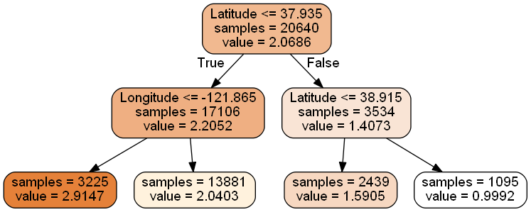
from sklearn import tree
dtr = tree.DecisionTreeRegressor(max_depth = 2)
dtr.fit(housing.data[:, [6, 7]], housing.target)

DecisionTreeRegressor(criterion='mse', max_depth=2, max_features=None,
           max_leaf_nodes=None, min_impurity_split=1e-07,
           min_samples_leaf=1, min_samples_split=2,
           min_weight_fraction_leaf=0.0, presort=False, random_state=None,
           splitter='best')

---

可视化 graphviz & pydotplus

#要可视化显示 首先需要安装 graphviz   http://www.graphviz.org/Download.php

dot_data = \
    tree.export_graphviz(
        dtr,
        out_file = None,
        feature_names = housing.feature_names[6:8],
        filled = True,
        impurity = False,
        rounded = True
    )

#pip install pydotplus
import pydotplus
graph = pydotplus.graph_from_dot_data(dot_data)
graph.get_nodes()[7].set_fillcolor("#FFF2DD")

from IPython.display import Image
Image(graph.create_png())

graph.write_png("dtr_white_background.png")   # 写入文件

---

from sklearn.model_selection import train_test_split
data_train, data_test, target_train, target_test = \
    train_test_split(housing.data, housing.target, test_size = 0.1, random_state = 42)
dtr = tree.DecisionTreeRegressor(random_state = 42)
dtr.fit(data_train, target_train)

dtr.score(data_test, target_test) # 0.637318351331017

from sklearn.ensemble import RandomForestRegressor
rfr = RandomForestRegressor( random_state = 42)
rfr.fit(data_train, target_train)
rfr.score(data_test, target_test)  # 0.79086492280964926

---

调整树模型参数

from sklearn.grid_search import GridSearchCV 

tree_param_grid = { 'min_samples_split': list((3,6,9)),'n_estimators':list((10,50,100))}
grid = GridSearchCV(RandomForestRegressor(),param_grid=tree_param_grid, cv=5)
grid.fit(data_train, target_train)
grid.grid_scores_, grid.best_params_, grid.best_score_

([mean: 0.78405, std: 0.00505, params: {'min_samples_split': 3, 'n_estimators': 10},
  mean: 0.80529, std: 0.00448, params: {'min_samples_split': 3, 'n_estimators': 50},
  mean: 0.80673, std: 0.00433, params: {'min_samples_split': 3, 'n_estimators': 100},
  mean: 0.79016, std: 0.00124, params: {'min_samples_split': 6, 'n_estimators': 10},
  mean: 0.80496, std: 0.00491, params: {'min_samples_split': 6, 'n_estimators': 50},
  mean: 0.80671, std: 0.00408, params: {'min_samples_split': 6, 'n_estimators': 100},
  mean: 0.78747, std: 0.00341, params: {'min_samples_split': 9, 'n_estimators': 10},
  mean: 0.80481, std: 0.00322, params: {'min_samples_split': 9, 'n_estimators': 50},
  mean: 0.80603, std: 0.00437, params: {'min_samples_split': 9, 'n_estimators': 100}],
 {'min_samples_split': 3, 'n_estimators': 100},
 0.8067250881273065)

rfr = RandomForestRegressor( min_samples_split=3,n_estimators = 100,random_state = 42)
rfr.fit(data_train, target_train)
rfr.score(data_test, target_test)  # 0.80908290496531576

pd.Series(rfr.feature_importances_, index = housing.feature_names).sort_values(ascending = False)
'''
 MedInc        0.524257
    AveOccup      0.137947
    Latitude      0.090622
    Longitude     0.089414
    HouseAge      0.053970
    AveRooms      0.044443
    Population    0.030263
    AveBedrms     0.029084
    dtype: float64
'''

---