


文章目录
相关文章:
Sklearn 支持向量机
Sklearn.svm 中用于分类的 SVM 方法:
-
svm.LinearSVC: Linear Support Vector Classification.
-
svm.NuSVC: Nu-Support Vector Classification.
-
svm.OneClassSVM: Unsupervised Outlier Detection.
-
svm.SVC: C-Support Vector Classification.
Sklearn.svm 中用于回归的 SVM 方法:
-
svm.LinearSVR: Linear Support Vector Regression.
-
svm.NuSVR: Nu Support Vector Regression.
-
svm.SVR: Epsilon-Support Vector Regression.
-
svm.l1_min_c: Return the lowest bound for C such that for C in (l1_min_C, infinity) the model is guaranteed not to be empty.
可以通过 model.support_vectors_ 查看支持向量。
SVM 对特征的缩放非常敏感,如下图所示,在左图中,垂直刻度比水平刻度大得多,因此可能的分离超平面接近于水平。在特征缩放后(如使用 Sklearn 的 StandardScaler)后(右图),决策边界看起来好看很多。
常用参数解释:
-
C C C:惩罚系数,用于近似线性数据中。在近似线性支持向量机中,损失函数由两部分组成:最大化支持向量间隔的大小以及 C × C\times C× 进入分类边界的数据点的惩罚大小。因此当 C C C 越大时,对进入边界的数据惩罚越大,表现为进入分类边界的数据越少(分类间隔越小)。 C C C 值的确定与问题有关,如医疗模型或垃圾邮件分类问题。
-
l o s s loss loss:损失函数。线性支持向量机中的目标函数可以分为两部分,第一部分为损失函数,第二部分为正则化项。默认的损失函数为合页损失函数(hinge loss function)
-
k e r n e l kernel kernel:非线性支持向量机中的核函数。常用的核函数由:线性核(即变为线性支持向量机)、多项式核、高斯 RBF 核、Sigmoid 核。
-
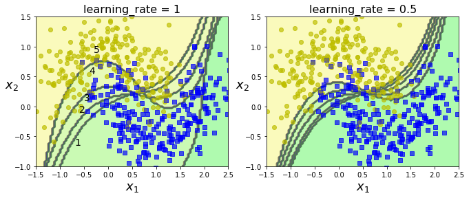
g a m m a gamma gamma:高斯核中的参数。 γ = 1 2 σ 2 \gamma = \frac{1}{2\sigma^2} γ=2σ21, σ \sigma σ 即正态分布中图像的横向宽度,所以 g a m m a gamma gamma 与 σ \sigma σ 呈反比,当 g a m m a gamma gamma 越大时,正态图越高瘦; g a m m a gamma gamma 越小时,正态图越矮胖。在 SVM 中表现如下:
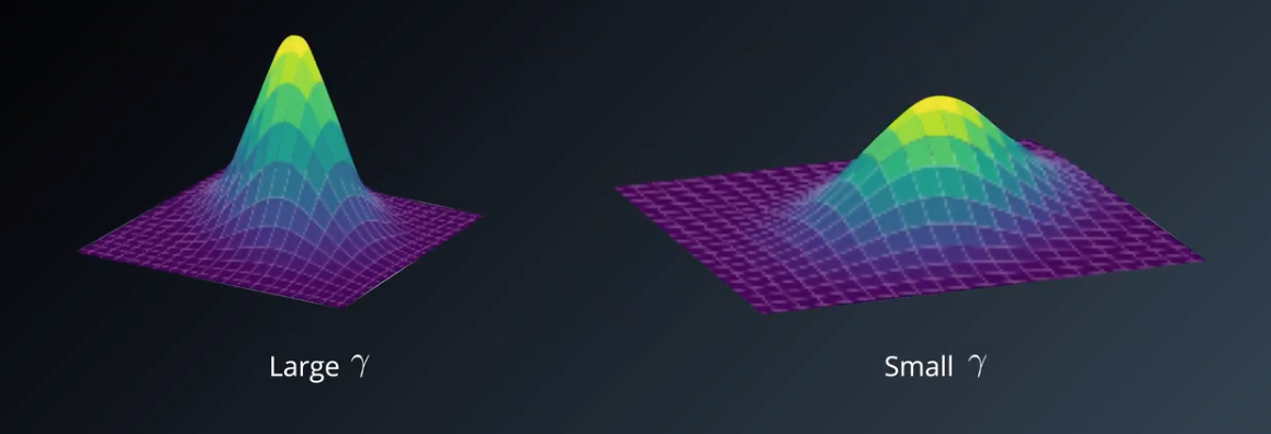
其截面为:
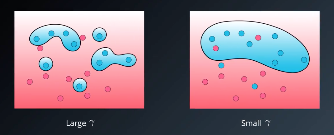
因此 gamma 越大,越可能过拟合; gamma 越小,越可能欠拟合。
1. 支持向量机分类
1.1 线性 SVM 分类
参数设置:
C: float, optional (default=1.0)
【惩罚参数,默认为1,C越大间隔越小,间隔中的实例也越少】
loss: string, ‘hinge’ or ‘squared_hinge’ (default=’squared_hinge’)
【loss 参数应设为 ‘hinge’ ,因为它不是默认值】
dual bool, (default=True)
【默认 True除非特征数量比训练实例还多,否则应设为 False】
其他参数见官方文档。
LinearSVC 类会对偏执项进行正则化,所以需要先减去平均值,使训练集集中。如果使用 StandardScaler 会自动进行这一步。
LinearSVC() 相当于 SVC(kernel=’linear’) ,但这要慢得多。
import numpy as np
from sklearn import datasets
from sklearn.pipeline import Pipeline
from sklearn.preprocessing import StandardScaler
from sklearn.svm import LinearSVC

iris = datasets.load_iris()
X = iris["data"][:, (2, 3)]  # petal length, petal width
y = (iris["target"] == 2).astype(np.float64)  # Iris-Virginica

svm_clf = Pipeline([
        ("scaler", StandardScaler()),
        ("linear_svc", LinearSVC(C=1, loss="hinge", random_state=42)),
    ])

svm_clf.fit(X, y)
Pipeline(memory=None,
         steps=[('scaler',
                 StandardScaler(copy=True, with_mean=True, with_std=True)),
                ('linear_svc',
                 LinearSVC(C=1, class_weight=None, dual=True,
                           fit_intercept=True, intercept_scaling=1,
                           loss='hinge', max_iter=1000, multi_class='ovr',
                           penalty='l2', random_state=42, tol=0.0001,
                           verbose=0))],
         verbose=False)
svm_clf.predict([[5.5, 1.7]])
array([1.])
与 Logistic 回归分类器不同的是,SVM 分类器不会输出每个类别的概率。
1.2 非线性 SVM 分类
虽然在许多情况下,线性 SVM 分类器是有效的,并且通常出人意料的好,但是,有很多数据集是非线性可分的。因此需要非线性支持向量机将数据变成线性可分的,如下图所示,利用多项式对数据进行变换:

要使用 Sklearn 实现这个想法,有两种方法:第一种是首先使用多项式变换并对特征进行缩放,接着就可以返回线性 linear_svc 分类器了;第二种是直接使用 SVC 分类器并选定多项式内核。
我们首先来看第一种,使用卫星数据来进行测试一下:
from sklearn.datasets import make_moons
import matplotlib.pyplot as plt

X, y = make_moons(n_samples=100, noise=0.15, random_state=42)

def plot_dataset(X, y, axes):
    plt.plot(X[:, 0][y==0], X[:, 1][y==0], "bs")
    plt.plot(X[:, 0][y==1], X[:, 1][y==1], "g^")
    plt.axis(axes)
    plt.grid(True, which='both')
    plt.xlabel(r"$x_1$", fontsize=20)
    plt.ylabel(r"$x_2$", fontsize=20, rotation=0)

plot_dataset(X, y, [-1.5, 2.5, -1, 1.5])
plt.show()
from sklearn.datasets import make_moons
from sklearn.pipeline import Pipeline
from sklearn.preprocessing import PolynomialFeatures

polynomial_svm_clf = Pipeline([
        ("poly_features", PolynomialFeatures(degree=3)),
        ("scaler", StandardScaler()),
        ("svm_clf", LinearSVC(C=10, loss="hinge", random_state=42))
    ])

polynomial_svm_clf.fit(X, y)
Pipeline(memory=None,
         steps=[('poly_features',
                 PolynomialFeatures(degree=3, include_bias=True,
                                    interaction_only=False, order='C')),
                ('scaler',
                 StandardScaler(copy=True, with_mean=True, with_std=True)),
                ('svm_clf',
                 LinearSVC(C=10, class_weight=None, dual=True,
                           fit_intercept=True, intercept_scaling=1,
                           loss='hinge', max_iter=1000, multi_class='ovr',
                           penalty='l2', random_state=42, tol=0.0001,
                           verbose=0))],
         verbose=False)
def plot_predictions(clf, axes):
    x0s = np.linspace(axes[0], axes[1], 100)
    x1s = np.linspace(axes[2], axes[3], 100)
    x0, x1 = np.meshgrid(x0s, x1s)
    X = np.c_[x0.ravel(), x1.ravel()]
    y_pred = clf.predict(X).reshape(x0.shape)
    y_decision = clf.decision_function(X).reshape(x0.shape)
    plt.contourf(x0, x1, y_pred, cmap=plt.cm.brg, alpha=0.2)
    plt.contourf(x0, x1, y_decision, cmap=plt.cm.brg, alpha=0.1)

plot_predictions(polynomial_svm_clf, [-1.5, 2.5, -1, 1.5])
plot_dataset(X, y, [-1.5, 2.5, -1, 1.5])

plt.show()
另外一种方法是使用 SVC 函数实现。
参数设置:
C: float, optional (default=1.0)
Penalty parameter C of the error term.
kernel: string, optional (default=’rbf’)
Specifies the kernel type to be used in the algorithm. It must be one of ‘linear’, ‘poly’, ‘rbf’, ‘sigmoid’, ‘precomputed’ or a callable. If none is given, ‘rbf’ will be used. If a callable is given it is used to pre-compute the kernel matrix from data matrices; that matrix should be an array of shape (n_samples, n_samples).
degree: int, optional (default=3)
Degree of the polynomial kernel function (‘poly’). Ignored by all other kernels.
gamma: {‘scale’, ‘auto’} or float, optional (default=’scale’)
Kernel coefficient for ‘rbf’, ‘poly’ and ‘sigmoid’.

if gamma='scale' (default) is passed then it uses 1 / (n_features * X.var()) as value of gamma,

if ‘auto’, uses 1 / n_features. Changed in version 0.22: The default value of gamma changed from ‘auto’ to ‘scale’.
coef0: float, optional (default=0.0)
Independent term in kernel function. It is only significant in ‘poly’ and ‘sigmoid’.

【控制模型受高阶多项式还是低阶多项式影响的程度】
其他参数设置见官方文档。
寻找正确的超参数值的常用方法是网络搜索。先进行一次粗略的网络搜索,然后在最好的值附近展开一轮更精细的网络搜索,这样通常会快一些。
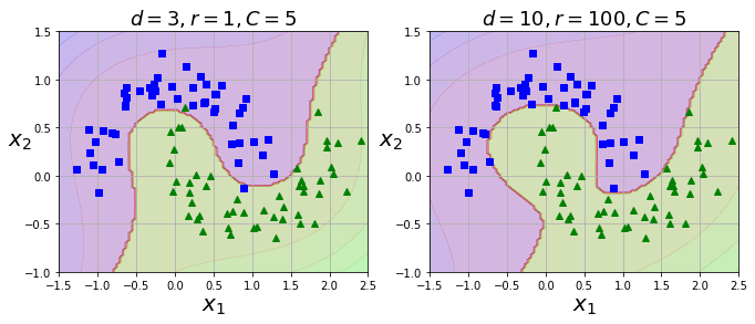
1.2.1 多项式内核
使用 SVC(kernel=“poly”, degree=3) 进行非线性多项式内核的 SVM 分类:
from sklearn.svm import SVC
from sklearn.datasets import make_moons
import matplotlib.pyplot as plt

X, y = make_moons(n_samples=100, noise=0.15, random_state=42)

poly_kernel_svm_clf = Pipeline([
        ("scaler", StandardScaler()),
        ("svm_clf", SVC(kernel="poly", degree=3, coef0=1, C=5))
    ])
poly_kernel_svm_clf.fit(X, y)
Pipeline(memory=None,
         steps=[('scaler',
                 StandardScaler(copy=True, with_mean=True, with_std=True)),
                ('svm_clf',
                 SVC(C=5, cache_size=200, class_weight=None, coef0=1,
                     decision_function_shape='ovr', degree=3,
                     gamma='auto_deprecated', kernel='poly', max_iter=-1,
                     probability=False, random_state=None, shrinking=True,
                     tol=0.001, verbose=False))],
         verbose=False)
poly100_kernel_svm_clf = Pipeline([
        ("scaler", StandardScaler()),
        ("svm_clf", SVC(kernel="poly", degree=10, coef0=100, C=5))
    ])
poly100_kernel_svm_clf.fit(X, y)
Pipeline(memory=None,
         steps=[('scaler',
                 StandardScaler(copy=True, with_mean=True, with_std=True)),
                ('svm_clf',
                 SVC(C=5, cache_size=200, class_weight=None, coef0=100,
                     decision_function_shape='ovr', degree=10,
                     gamma='auto_deprecated', kernel='poly', max_iter=-1,
                     probability=False, random_state=None, shrinking=True,
                     tol=0.001, verbose=False))],
         verbose=False)
plt.figure(figsize=(11, 4))

plt.subplot(121)
plot_predictions(poly_kernel_svm_clf, [-1.5, 2.5, -1, 1.5])
plot_dataset(X, y, [-1.5, 2.5, -1, 1.5])
plt.title(r"$d=3, r=1, C=5$", fontsize=18)

plt.subplot(122)
plot_predictions(poly100_kernel_svm_clf, [-1.5, 2.5, -1, 1.5])
plot_dataset(X, y, [-1.5, 2.5, -1, 1.5])
plt.title(r"$d=10, r=100, C=5$", fontsize=18)

plt.show()
1.2.2 高斯 RBF 内核
使用 SVC(kernel=‘rbf’, gamma=5, C=0.001) 对非线性数据进行分类:
from sklearn.datasets import make_moons
import matplotlib.pyplot as plt

X, y = make_moons(n_samples=100, noise=0.15, random_state=42)

rbf_kernel_svm_clf = Pipeline([
        ("scaler", StandardScaler()),
        ("svm_clf", SVC(kernel="rbf", gamma=5, C=0.001))
    ])
rbf_kernel_svm_clf.fit(X, y)
Pipeline(memory=None,
         steps=[('scaler',
                 StandardScaler(copy=True, with_mean=True, with_std=True)),
                ('svm_clf',
                 SVC(C=0.001, cache_size=200, class_weight=None, coef0=0.0,
                     decision_function_shape='ovr', degree=3, gamma=5,
                     kernel='rbf', max_iter=-1, probability=False,
                     random_state=None, shrinking=True, tol=0.001,
                     verbose=False))],
         verbose=False)
实现简单的网络搜索:
from sklearn.svm import SVC

gamma1, gamma2 = 0.1, 5
C1, C2 = 0.001, 1000
hyperparams = (gamma1, C1), (gamma1, C2), (gamma2, C1), (gamma2, C2)

svm_clfs = []
for gamma, C in hyperparams:
    rbf_kernel_svm_clf = Pipeline([
            ("scaler", StandardScaler()),
            ("svm_clf", SVC(kernel="rbf", gamma=gamma, C=C))
        ])
    rbf_kernel_svm_clf.fit(X, y)
    svm_clfs.append(rbf_kernel_svm_clf)

plt.figure(figsize=(11, 7))

for i, svm_clf in enumerate(svm_clfs):
    plt.subplot(221 + i)
    plot_predictions(svm_clf, [-1.5, 2.5, -1, 1.5])
    plot_dataset(X, y, [-1.5, 2.5, -1, 1.5])
    gamma, C = hyperparams[i]
    plt.title(r"$\gamma = {}, C = {}$".format(gamma, C), fontsize=16)

plt.show()

2. 支持向量机回归
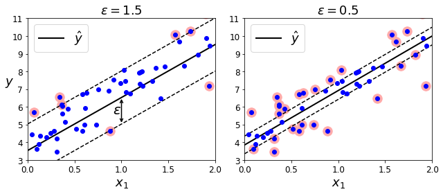
SVM 算法非常全面:它不仅支持线性和非线性分类,而且还支持线性和非线性回归。诀窍在于将目标反转一下:不再是尝试拟合最大分离间隔,SVM 回归要做的是让尽可能多的实例位于间隔中间,同时限制间隔违例。间隔的宽度受超参数 ε \varepsilon ε 控制。
2.1 线性 SVM 回归
sklearn.svm.LinearSVR (训练数据需要先缩放并集中)
参数设置:
epsilon: float, optional (default=0.0)
Epsilon parameter in the epsilon-insensitive loss function. Note that the value of this parameter depends on the scale of the target variable y. If unsure, set epsilon=0.
【间隔宽度】
tol: float, optional (default=1e-4)
Tolerance for stopping criteria.
C: float, optional (default=1.0)
Penalty parameter C of the error term. The penalty is a squared l2 penalty. The bigger this parameter, the less regularization is used.
loss: string, optional (default=’epsilon_insensitive’)
Specifies the loss function. The epsilon-insensitive loss (standard SVR) is the L1 loss, while the squared epsilon-insensitive loss (‘squared_epsilon_insensitive’) is the L2 loss.
dual: bool, (default=True)
Select the algorithm to either solve the dual or primal optimization problem. Prefer dual=False when n_samples > n_features.
from sklearn.svm import LinearSVR

linear_svm_reg = Pipeline([
        ("scaler", StandardScaler()),
        ("svm_reg", LinearSVR(epsilon=1.5))
    ])
linear_svm_reg.fit(X, y)
下图显示了用随机线性数据训练的两个线性 SVM回归模型,一个间隔较大( ε = 1.5 \varepsilon=1.5 ε=1.5 ),一个间隔较小( ε = 0.5 \varepsilon=0.5 ε=0.5 )(训练数据需要先缩放并集中)。
绘图代码:
np.random.seed(42)
m = 50
X = 2 * np.random.rand(m, 1)
y = (4 + 3 * X + np.random.randn(m, 1)).ravel()
from sklearn.svm import LinearSVR

svm_reg = LinearSVR(epsilon=1.5, random_state=42)
svm_reg.fit(X, y)
LinearSVR(C=1.0, dual=True, epsilon=1.5, fit_intercept=True,
          intercept_scaling=1.0, loss='epsilon_insensitive', max_iter=1000,
          random_state=42, tol=0.0001, verbose=0)
svm_reg1 = LinearSVR(epsilon=1.5, random_state=42)
svm_reg2 = LinearSVR(epsilon=0.5, random_state=42)
svm_reg1.fit(X, y)
svm_reg2.fit(X, y)

def find_support_vectors(svm_reg, X, y):
    y_pred = svm_reg.predict(X)
    off_margin = (np.abs(y - y_pred) >= svm_reg.epsilon)
    return np.argwhere(off_margin)

svm_reg1.support_ = find_support_vectors(svm_reg1, X, y)
svm_reg2.support_ = find_support_vectors(svm_reg2, X, y)

eps_x1 = 1
eps_y_pred = svm_reg1.predict([[eps_x1]])
def plot_svm_regression(svm_reg, X, y, axes):
    x1s = np.linspace(axes[0], axes[1], 100).reshape(100, 1)
    y_pred = svm_reg.predict(x1s)
    plt.plot(x1s, y_pred, "k-", linewidth=2, label=r"$\hat{y}$")
    plt.plot(x1s, y_pred + svm_reg.epsilon, "k--")
    plt.plot(x1s, y_pred - svm_reg.epsilon, "k--")
    plt.scatter(X[svm_reg.support_], y[svm_reg.support_], s=180, facecolors='#FFAAAA')
    plt.plot(X, y, "bo")
    plt.xlabel(r"$x_1$", fontsize=18)
    plt.legend(loc="upper left", fontsize=18)
    plt.axis(axes)

plt.figure(figsize=(9, 4))
plt.subplot(121)
plot_svm_regression(svm_reg1, X, y, [0, 2, 3, 11])
plt.title(r"$\epsilon = {}$".format(svm_reg1.epsilon), fontsize=18)
plt.ylabel(r"$y$", fontsize=18, rotation=0)
#plt.plot([eps_x1, eps_x1], [eps_y_pred, eps_y_pred - svm_reg1.epsilon], "k-", linewidth=2)
plt.annotate(
        '', xy=(eps_x1, eps_y_pred), xycoords='data',
        xytext=(eps_x1, eps_y_pred - svm_reg1.epsilon),
        textcoords='data', arrowprops={'arrowstyle': '<->', 'linewidth': 1.5}
    )
plt.text(0.91, 5.6, r"$\epsilon$", fontsize=20)
plt.subplot(122)
plot_svm_regression(svm_reg2, X, y, [0, 2, 3, 11])
plt.title(r"$\epsilon = {}$".format(svm_reg2.epsilon), fontsize=18)
plt.show()
2.2 非线性 SVM 回归
参数设置:
kernel: string, optional (default=’rbf’)
Specifies the kernel type to be used in the algorithm. It must be one of ‘linear’, ‘poly’, ‘rbf’, ‘sigmoid’, ‘precomputed’ or a callable. If none is given, ‘rbf’ will be used. If a callable is given it is used to precompute the kernel matrix.
degree: int, optional (default=3)
Degree of the polynomial kernel function (‘poly’). Ignored by all other kernels.
gamma: {‘scale’, ‘auto’} or float, optional
(default=’scale’)
Kernel coefficient for ‘rbf’, ‘poly’ and ‘sigmoid’.

if gamma='scale' (default) is passed then it uses 1 / (n_features * X.var()) as value of gamma,

if ‘auto’, uses 1 / n_features.

Changed in version 0.22: The default value of gamma changed from ‘auto’ to ‘scale’.
coef0: float, optional (default=0.0)
Independent term in kernel function. It is only significant in ‘poly’ and ‘sigmoid’.
tol: float, optional (default=1e-3)
Tolerance for stopping criterion.
C: float, optional (default=1.0)
Penalty parameter C of the error term.
epsilon: float, optional (default=0.1)
Epsilon in the epsilon-SVR model. It specifies the epsilon-tube within which no penalty is associated in the training loss function with points predicted within a distance epsilon from the actual value.
【它指定了epsilon-tube,其中训练损失函数中没有惩罚与在实际值的距离epsilon内预测的点。】
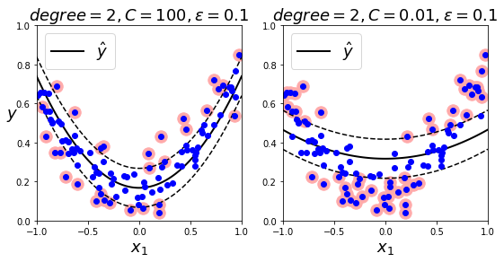
2.2.1 多项式内核
from sklearn.svm import SVR

svm_poly_reg = SVR(kernel="poly", degree=2, C=100, epsilon=0.1, gamma="auto")
svm_poly_reg.fit(X, y)
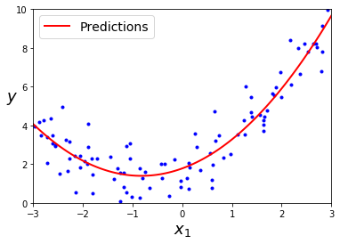
下面展示了不同惩罚系数(C)下的 SVM 回归:
代码如下:
np.random.seed(42)
m = 100
X = 2 * np.random.rand(m, 1) - 1
y = (0.2 + 0.1 * X + 0.5 * X**2 + np.random.randn(m, 1)/10).ravel()
设置不同的正则化值(C 值)
from sklearn.svm import SVR

svm_poly_reg1 = SVR(kernel="poly", degree=2, C=100, epsilon=0.1, gamma="auto")
svm_poly_reg2 = SVR(kernel="poly", degree=2, C=0.01, epsilon=0.1, gamma="auto")
svm_poly_reg1.fit(X, y)
svm_poly_reg2.fit(X, y)
SVR(C=0.01, cache_size=200, coef0=0.0, degree=2, epsilon=0.1, gamma='auto',
    kernel='poly', max_iter=-1, shrinking=True, tol=0.001, verbose=False)
import matplotlib.pyplot as plt
def plot_svm_regression(svm_reg, X, y, axes):
    x1s = np.linspace(axes[0], axes[1], 100).reshape(100, 1)
    y_pred = svm_reg.predict(x1s)
    plt.plot(x1s, y_pred, "k-", linewidth=2, label=r"$\hat{y}$")
    plt.plot(x1s, y_pred + svm_reg.epsilon, "k--")
    plt.plot(x1s, y_pred - svm_reg.epsilon, "k--")
    plt.scatter(X[svm_reg.support_], y[svm_reg.support_], s=180, facecolors='#FFAAAA')
    plt.plot(X, y, "bo")
    plt.xlabel(r"$x_1$", fontsize=18)
    plt.legend(loc="upper left", fontsize=18)
    plt.axis(axes)
plt.figure(figsize=(9, 4))
plt.subplot(121)
plot_svm_regression(svm_poly_reg1, X, y, [-1, 1, 0, 1])
plt.title(r"$degree={}, C={}, \epsilon = {}$".format(svm_poly_reg1.degree, svm_poly_reg1.C, svm_poly_reg1.epsilon), fontsize=18)
plt.ylabel(r"$y$", fontsize=18, rotation=0)
plt.subplot(122)
plot_svm_regression(svm_poly_reg2, X, y, [-1, 1, 0, 1])
plt.title(r"$degree={}, C={}, \epsilon = {}$".format(svm_poly_reg2.degree, svm_poly_reg2.C, svm_poly_reg2.epsilon), fontsize=18)
plt.show()
参考资料
[1] Aurelien Geron, 王静源, 贾玮, 边蕤, 邱俊涛. 机器学习实战:基于 Scikit-Learn 和 TensorFlow[M]. 北京: 机械工业出版社, 2018: 136-144.


 547
547


 被折叠的 条评论
为什么被折叠?
被折叠的 条评论
为什么被折叠?
 到【灌水乐园】发言


