


TensorFlow1.9卷积神经网络
一、卷积神经网络理论基础
1.卷积神经网络介绍
- 卷积神经网络主要用于图像处理相关的任务
- 典型图像处理相关任务包括分类、定位、检测、分割
- 对于计算机来说,图像由矩阵表示,图像处理任务即处理矩阵
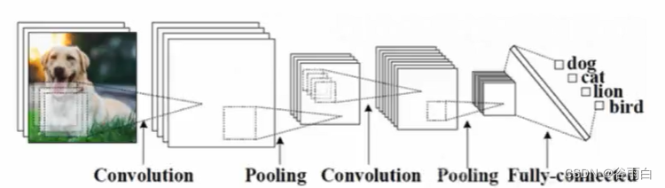
2.卷积网络的基本组成
- 卷积层:提取特征,形成特征图
- 池化层:压缩特征图,减少计算复杂度,提取主要特征
- 全连接层:连接所有的特征,将输出值传给分类器(Softmax)
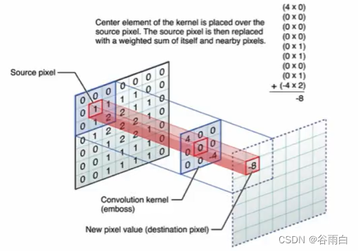
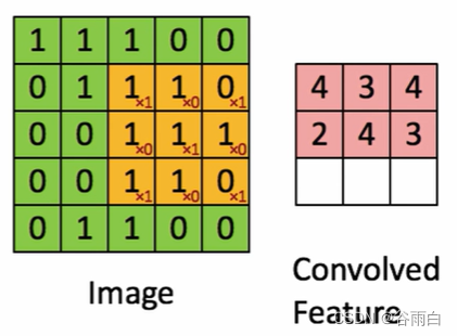
3.卷积操作详解
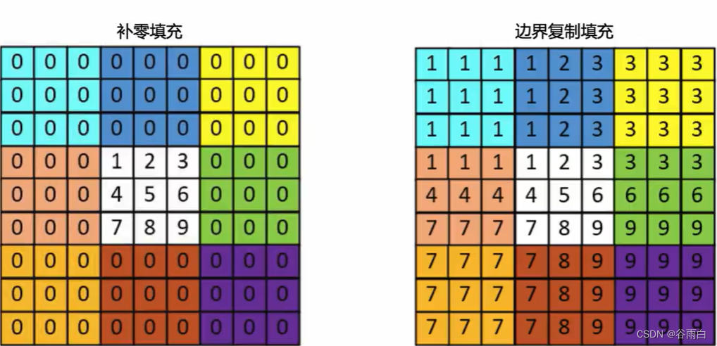
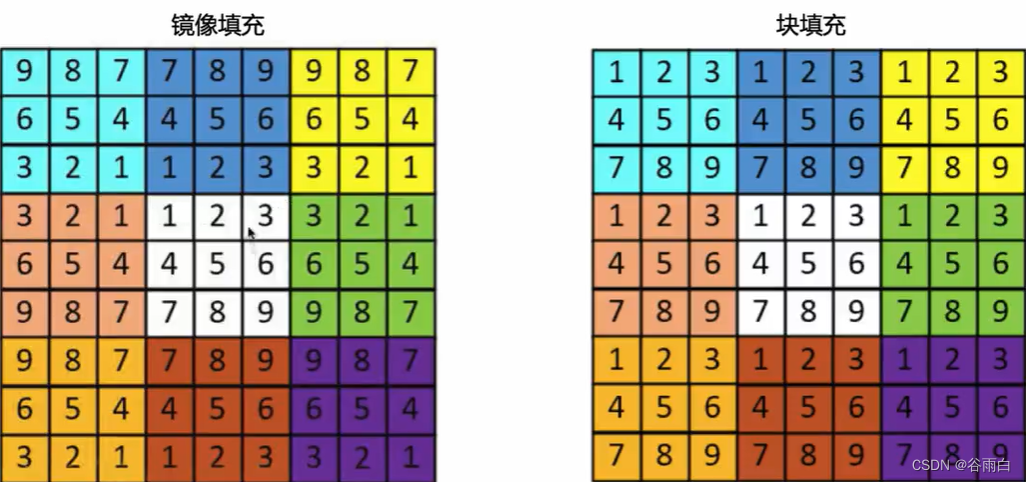
4.卷积的边界补充
二、卷积核、池化
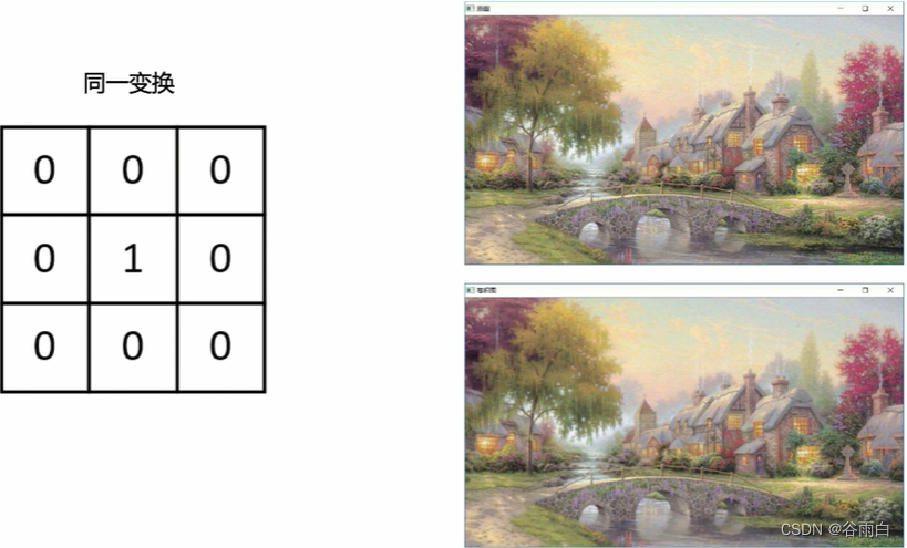
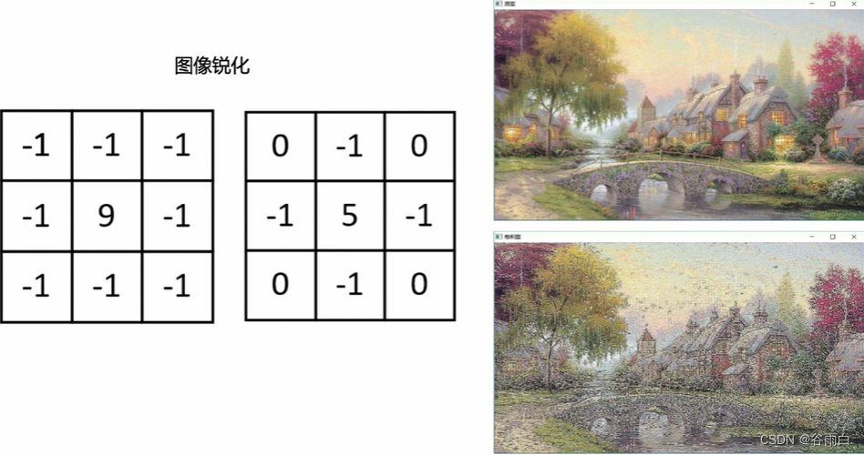
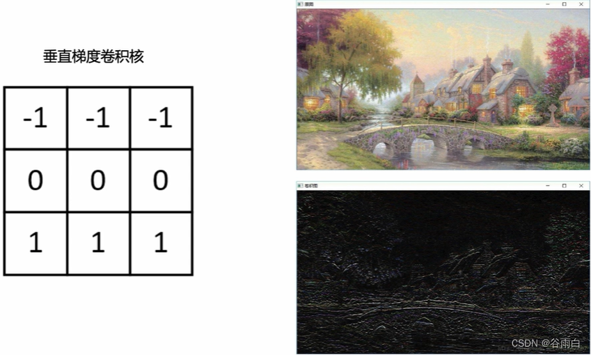
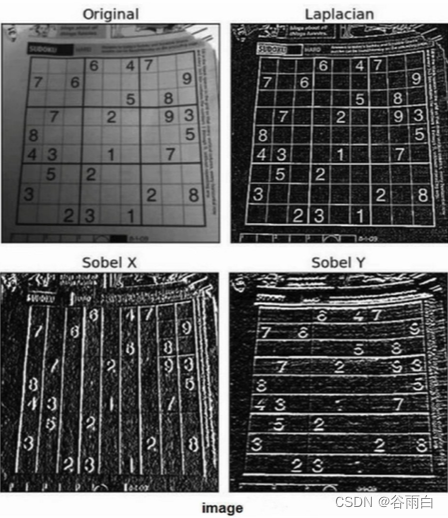
1.不同卷积核的意义
- 高斯滤波:平滑 去噪

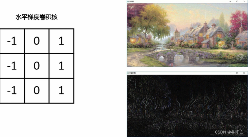
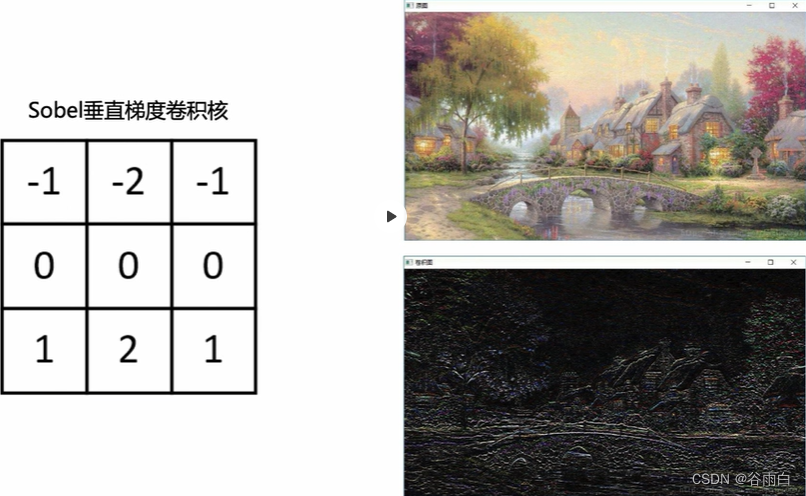
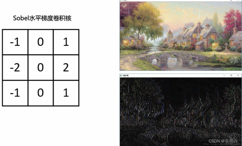
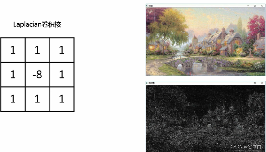
- 边缘提取:水平梯度卷积核 垂直梯度卷积核 sobel水平梯度卷积核 sobel垂直梯度卷积核 Laplacian卷积核
2.卷积层
- 卷积层通对卷积核对图像进行卷积操作
- 卷积核又称滤波器,在神经网络里代表权重,用于提取图像的特征
- 卷积层涉及的参数一般包括卷积核数目、大小、步长、边界补充策略(padding)
- 除了指定padding的层数,实际运用中、在"valid"和"same“两种策略
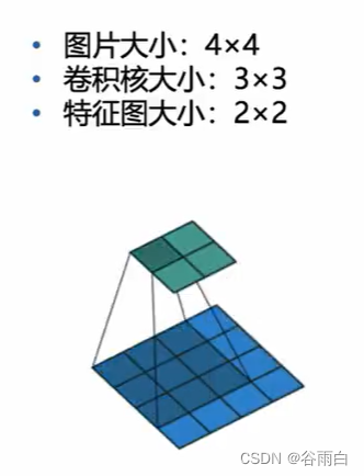
3.卷积后图片大小的计算
- 输入图片尺寸wxw
- 卷积核大小FxF
- 步长s
- Padding层数P
- 输出图片大小NxN
- N=(w -F+2P)/S +1
- 若padding = “valid”,此时不会padding新的像素,输出N=(W-F+1)/S(向上取整)
- 若padding = "same”,此时输入会进行补零填充,此时输出只和步长有关,输出N=W/S(向上取整)
4.池化层
- 在卷积层之后,往往会接一个池化层,池化层是一个下采样过程
- 常见的池化层有最大值池化,均值池化,随机池化等
- 池化层的作用包括特征不变性、特征降维、防止过拟合等
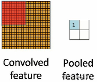
- 下图展示了最大值池化和平均值池化的过程
- 一般来说池化层所需参数与卷积层相同
- 池化层的padding策略与卷积层一致,一般分为"valid"和"same"
- 下图采用2×2的卷积核,步长为2, padding策略为"valid"
三.CNN的基本结构
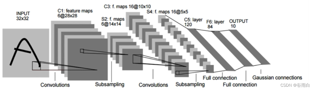
1.LeNwt-5的基本结构
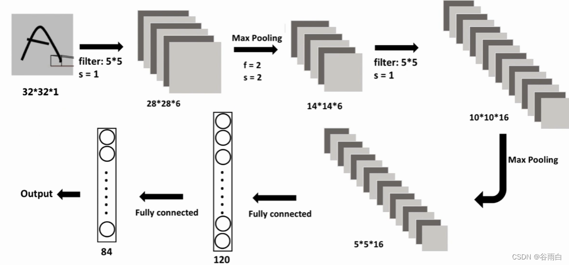
- 以LeNet-5为例,其被设计用来实现图像分类任务,其中包含了卷积层、池化层与全连接层
- 输入数据为32×32,经过一个卷积核为5x5,步长为1,padding策略为“valid"的卷积层,由公式N=(w -F+0)/S+1=(32-5+0)/1+1= 28,计算得出卷积后图像大小为28×28
- 经过第一层卷积后的图像经过一个大小为2×2,步长为2的池化层,padding策略是"same”,故经过池化后图像大小变为原来四分之一,即14×14,后续的卷积池化同理
四、MNIST CNN Tensorflow
1.构建CNN用的到的基本Tensorflow函数
#输入与参数
tf.placeholder
tf.nn.conv2d

#初始化方法
tf.random_normal

#CNN基本函数
tf.nn.conv2d #2d卷积层
tf.nn.relu 	  #relu激活函数
tf.nn. max_pool #最大值池化层
tf.reshape      #调整张量维度
tf.matmul       #矩阵乘法
tf.nn.dropout   #dropout层

#训练相关函数
tf.nn. softmax_cross_entropy_with_logits #交叉熵损失函数
tf.train.AdamOptimizer                   #Adam优化器
tf.reduce_mean                           #计算张量指定轴方向的均值
2.实例1(识别mnist手写数据集)
# In[]
# 载入数据
import tensorflow as tf
from tensorflow.examples.tutorials.mnist import input_data
# 对标签进行One-Hot编码
mnist = input_data.read_data_sets("MNIST_data", one_hot = True)
# In[]
# 参数设置
n_classes = 10  # 分类的类别
batch_size = 100  # batch的大小
# In[]
# 定义占位符
x = tf.placeholder('float', [None, 28*28])
y = tf.placeholder('float')

# In[]
# 定义卷积层计算,步长为1,填充策略为SAME
def conv2d(x, W):
    return tf.nn.conv2d(x, W, strides=[1, 1, 1, 1], padding='SAME')


# In[]
# 定义池化层计算,步长为2,填充策略为SAME
def maxpool2d(x):
    return tf.nn.max_pool(x, ksize=[1, 2, 2, 1], strides=[1, 2, 2, 1], padding='SAME')


# In[]
# 定义网络结构及计算过程
def neural_network_model(data):
    # 图像大小 28*28 -- 14*14 -- 7*7
    # 采用字典定义网络结构
    weights = {
        # 卷积层1的权重,32个5×5卷积核
        'W_conv1': tf.Variable(tf.random_normal([5, 5, 1, 32])),
        # 卷积层2的权重,64个5×5卷积核
        'W_conv2': tf.Variable(tf.random_normal([5, 5, 32, 64])),
        # 全连接层,1024个神经元
        'W_fc': tf.Variable(tf.random_normal([7*7*64, 1024])),
        # 输出层,10个神经元
        'out': tf.Variable(tf.random_normal([1024, n_classes]))
    }

    biases = {
        # 卷积层1的偏置,共32个
        'b_conv1': tf.Variable(tf.random_normal([32])),
        # 卷积层2的偏置,共64个
        'b_conv2': tf.Variable(tf.random_normal([64])),
        # 全连接层的偏置,共1024个
        'b_fc': tf.Variable(tf.random_normal([1024])),
        # 输出层的偏置,共10个
        'out': tf.Variable(tf.random_normal([n_classes]))
    }
    # 数据维度转化
    data = tf.reshape(data, [-1, 28, 28, 1])

    # 每层计算过程
    # 卷积层1,卷积+池化
    conv1 = tf.nn.relu(conv2d(data, weights['W_conv1']) + biases['b_conv1'])
    conv1 = maxpool2d(conv1)

    # 卷积层2,卷积+池化
    conv2 = tf.nn.relu(conv2d(conv1, weights['W_conv2']) + biases['b_conv2'])
    conv2 = maxpool2d(conv2)

    # 全连接层
    fc = tf.reshape(conv2, [-1, 7*7*64])
    fc = tf.nn.relu(tf.matmul(fc, weights['W_fc']) + biases['b_fc'])

    # 输出层,无需经过Softmax,只需计算加权和
    output = tf.matmul(fc, weights['out']) + biases['out']

    return output


# In[]
# 实现网络的训练和验证
def train_neural_network(x):
    prediction = neural_network_model(x)

    # 定义损失函数与优化器
    ## 平均Softmax对数交叉熵损失,需要输入输出层的输出结果和经过One-Hot处理的标签
    cost = tf.reduce_mean(tf.nn.softmax_cross_entropy_with_logits(logits = prediction, labels = y))
    ## 优化方法为Adam
    optimizer = tf.train.AdamOptimizer().minimize(cost)

    # 迭代10轮
    hm_epochs = 10
    with tf.Session() as sess:
        # 参数初始化
        sess.run(tf.global_variables_initializer())

        for epoch in range(hm_epochs):
            epoch_loss = 0 # 累计损失
            for _ in range(int(mnist.train.num_examples / batch_size)):
                # 提取数据
                epoch_x, epoch_y = mnist.train.next_batch(batch_size)
                # 喂数据
                _, c = sess.run([optimizer, cost], feed_dict= {x: epoch_x, y: epoch_y})
                epoch_loss = epoch_loss + c

            print('Epoch', epoch, 'completed out of', hm_epochs, 'loss', epoch_loss)
        # 计算分类正确率
        correct = tf.equal(tf.argmax(prediction, 1), tf.argmax(y, 1))
        accuracy = tf.reduce_mean(tf.cast(correct, 'float'))
        print('Accuracy:', accuracy.eval({x: mnist.test.images, y: mnist.test.labels}))

# 进行训练
train_neural_network(x)
实例2(minist服饰)
# -*- coding: utf-8 -*-
# 载入所需要的包
# In[]
from tensorflow import keras
import tensorflow as tf
import numpy as np
from matplotlib import pyplot as plt
# In[]
# fasin mnist
fashion_mnist = keras.datasets.fashion_mnist
(train_images,train_labels),(test_images,test_labels)=fashion_mnist.load_data()
# In[]
print(train_images.shape)
# In[]
plt.figure()
plt.imshow(train_images[0])
plt.colorbar()
plt.grid(False)
plt.show()

# In[]
train_images=train_images/255.0
test_images=test_images/255.0
# In[]
class_names=["T-shirt/top","Trouser","Pullover","Dress","Coat","sandal","shirt","sneaker","bag","ankel"]
plt.figure(figsize=(10,10))
for i in range(25):
    plt.subplot(5,5,i+1)
    plt.xticks([])
    plt.yticks([])
    plt.grid(False)
    plt.imshow(train_images[i],cmap=plt.cm.binary)
    plt.xlabel(class_names[train_labels[i]])
plt.show()

# In[]
#Model define
#MLP
model = keras.Sequential([
    keras.layers.Flatten(input_shape=(28,28)),
    keras.layers.Dense(128,activation=tf.nn.relu),
    keras.layers.Dense(10,activation=tf.nn.softmax)
    ])

# In[]
print(train_labels.shape)
# In[]
# CNN
train_images=train_images.reshape(60000,28,28,1)

model=keras.Sequential([
    keras.layers.Conv2D(32,kernel_size=(5,5),strides=(1,1),activation="relu",input_shape=(28,28,1)),
    keras.layers.MaxPooling2D(pool_size=(2,2),strides=(2,2)),
    keras.layers.Conv2D(64,kernel_size=(5,5),strides=(1,1),activation="relu"),
    keras.layers.MaxPooling2D(pool_size=(2,2),strides=(2,2)),
    keras.layers.Flatten(),
    keras.layers.Dense(1000,activation="relu"),
    keras.layers.Dropout(0.5),
    keras.layers.Dense(10,activation="softmax")
    ])
# In[]
model.summary()
# In[]
model.compile(optimizer="adam",loss="sparse_categorical_crossentropy",metrics=['categorical_accuracy'])

# In[]
model.fit(train_images,train_labels,epochs=10)

# In[]
test_loss,test_acc=model.evaluate(test_images,test_labels)

print("Test Accuracy:",test_acc)

# In[]
#model prediction
predictions=model.predict(test_images)


 311
311


 被折叠的 条评论
为什么被折叠?
被折叠的 条评论
为什么被折叠?
 到【灌水乐园】发言


