一、直方图相关学习

我是个菜鸡.

已于 2024-02-27 22:01:24 修改

阅读量498

点赞数 9

文章标签：学习 opencv 计算机视觉

于 2024-02-18 22:36:11 首次发布

本文链接：https://blog.csdn.net/weixin_45988242/article/details/136158075

版权

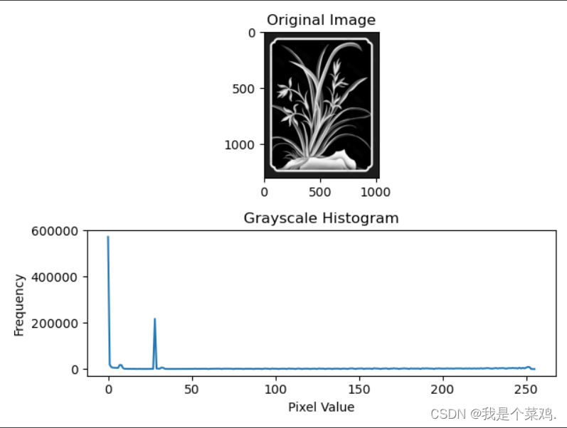
1、灰度直方图

1.1 基本概念和作用

表示图像中每个灰度级别的像素数量。用于分析图像的亮度分布情况。

1.2 代码示例

参数介绍

hist = cv2.calcHist(images, channels, mask, histSize, ranges, hist, accumulate)

-images：输入图像的列表。对于灰度图像，它只包含一个元素（即一幅图像）。对于彩色图像，通常会传入一个包含所有颜色通道的列表。
-channels：指定要统计直方图的通道。对于灰度图像，值为[0]；对于彩色图像，可以传入[0]、[1]、[2]分别表示蓝、绿、红通道。如果是彩色图像，也可以同时统计多个通道，例如[0, 1, 2]表示统计所有通道。
-mask：可选参数，用于指定计算直方图的区域。如果不需要指定区域，传入None
-histSize：指定直方图的大小，即灰度级别的个数。对于灰度图像，通常设置为256，表示从0到255的灰度级别。对于彩色图像，可以设置为256，表示每个通道的灰度级别。
-ranges：指定像素值的范围。通常为[0, 256]，表示灰度级别的范围。对于彩色图像，例如[0, 256, 0, 256, 0, 256]表示三个通道各自的范围。
-hist：可选参数，用于存储计算得到的直方图。如果不提供，函数会返回直方图
-accumulate：

示例

import cv2
import matplotlib.pyplot as plt

# 读取图像
image = cv2.imread('../images/1.jpg', cv2.IMREAD_GRAYSCALE)

# 计算灰度直方图
hist = cv2.calcHist([image], [0], None, [256], [0, 256])

# 显示原图
plt.subplot(2, 1, 1)
plt.imshow(image, cmap='gray')
plt.title('Original Image')

# 显示灰度直方图
plt.subplot(2, 1, 2)
plt.plot(hist)
plt.title('Grayscale Histogram')
plt.xlabel('Pixel Value')
plt.ylabel('Frequency')

# 调整子图布局，避免重叠
plt.tight_layout()

# 显示图像和直方图
plt.show()

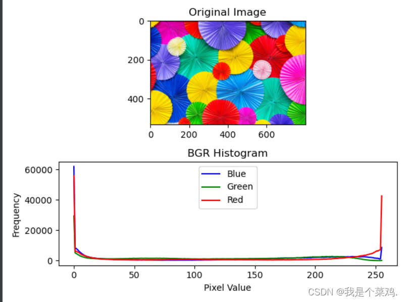
2、BGR直方图

2.1 基本概念和作用

BGR直方图是一种用于可视化彩色图像中蓝色（Blue）、绿色（Green）和红色（Red）三个通道的像素值分布情况的工具。了解图像中颜色的分布情况。通过分析BGR直方图，可以得知图像中某个颜色通道的强度，从而更好地理解图像的颜色特性。

2.2 代码示例

import cv2
import matplotlib.pyplot as plt

# 读取彩色图像
image = cv2.imread('../images/2.jpg')

# 分离通道
b, g, r = cv2.split(image)

# 计算各通道的直方图
hist_b = cv2.calcHist([b], [0], None, [256], [0, 256])
hist_g = cv2.calcHist([g], [0], None, [256], [0, 256])
hist_r = cv2.calcHist([r], [0], None, [256], [0, 256])

# 显示彩色图像
plt.subplot(2, 1, 1)
plt.imshow(cv2.cvtColor(image, cv2.COLOR_BGR2RGB))
plt.title('Original Image')

# 显示BGR直方图
plt.subplot(2, 1, 2)
plt.plot(hist_b, color='blue', label='Blue')
plt.plot(hist_g, color='green', label='Green')
plt.plot(hist_r, color='red', label='Red')
plt.title('BGR Histogram')
plt.xlabel('Pixel Value')
plt.ylabel('Frequency')
plt.legend()

# 调整子图布局，避免重叠
plt.tight_layout()
# 显示图像和直方图
plt.show()

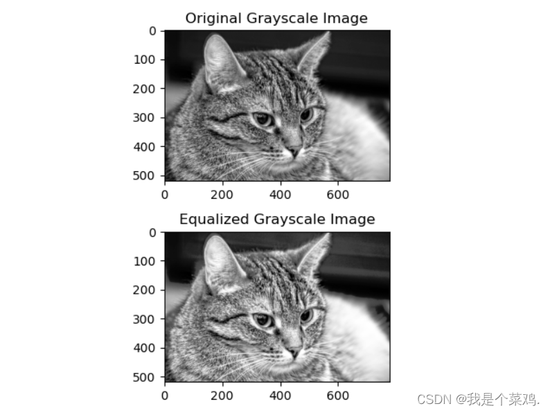
3、灰度直方图均衡

1. 基本概念和作用

用于增强图像对比度的技术，通过调整图像中各个灰度级别的像素分布，使得整个灰度范围更均匀地覆盖，从而提高图像的视觉质量。这个过程可以使暗部和亮部细节更加清晰可见，改善图像的视觉效果。

2. 代码示例

import cv2
import matplotlib.pyplot as plt

# 读取灰度图像
image = cv2.imread('../images/3.jpg', cv2.IMREAD_GRAYSCALE)

# 进行灰度直方图均衡
equalized_image = cv2.equalizeHist(image)

# 显示原始灰度图像
plt.subplot(2, 1, 1)
plt.imshow(image, cmap='gray')
plt.title('Original Grayscale Image')

# 显示均衡后的灰度图像
plt.subplot(2, 1, 2)
plt.imshow(equalized_image, cmap='gray')
plt.title('Equalized Grayscale Image')

# 调整子图布局，避免重叠
plt.tight_layout()

# 显示图像
plt.show()

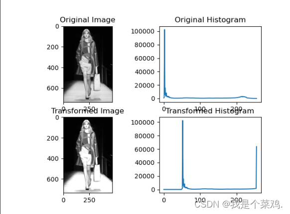
4、直方图变换（查找）

4.1 基本概念和作用

直方图变换，也称为直方图查找，是一种用于调整图像对比度的技术。它通过变换图像的灰度级别，将原始图像的灰度分布均匀化，使得图像中所有灰度级别的像素值分布更加平均。这样可以增强图像的对比度，使细节更加突出，提高图像的视觉质量。
直方图变换的核心思想是调整图像中各个灰度级别的像素值，使得灰度值的分布更均匀，从而实现对比度的增强。

4.2 代码示例

import cv2
import numpy as np
import matplotlib.pyplot as plt

# 读取图像
img = cv2.imread('../images/4.jpg', cv2.IMREAD_GRAYSCALE)

# 计算原始图像的直方图
hist = cv2.calcHist([img], [0], None, [256], [0, 256])

# 显示原始图像和直方图
plt.subplot(2, 2, 1), plt.imshow(img, cmap='gray'), plt.title('Original Image')
plt.subplot(2, 2, 2), plt.plot(hist), plt.title('Original Histogram')

# 构建查找表，每个像素值增加50
lookup_table = np.arange(256, dtype=np.uint8)
lookup_table = cv2.add(lookup_table, 50)

# 应用查找表
transformed_img = cv2.LUT(img, lookup_table)

# 计算变换后图像的直方图
transformed_hist = cv2.calcHist([transformed_img], [0], None, [256], [0, 256])

# 显示变换后图像和直方图
plt.subplot(2, 2, 3), plt.imshow(transformed_img, cmap='gray'), plt.title('Transformed Image')
plt.subplot(2, 2, 4), plt.plot(transformed_hist), plt.title('Transformed Histogram')

plt.show()

图片中每个像素都增加五十个像素的效果

5、直方图匹配

5.1 基本概念和作用

通过调整图像的像素值，使其直方图匹配到另一图像的直方图，以实现两者视觉特性的一致性。在图像配准、图像融合等应用

5.2 代码示例

import cv2
import matplotlib.pyplot as plt
import numpy as np

def hist_match(source, target):
    # 将源图像和目标图像转换为灰度图
    source_gray = cv2.cvtColor(source, cv2.COLOR_BGR2GRAY)
    target_gray = cv2.cvtColor(target, cv2.COLOR_BGR2GRAY)

    # 计算源图像和目标图像的直方图
    source_hist, _ = np.histogram(source_gray.flatten(), 256, [0, 256])
    target_hist, _ = np.histogram(target_gray.flatten(), 256, [0, 256])

    # 直方图归一化
    source_hist = source_hist / source_hist.sum()
    target_hist = target_hist / target_hist.sum()

    # 计算累积分布函数（CDF）
    source_cdf = source_hist.cumsum()
    target_cdf = target_hist.cumsum()

    # 映射源图像的像素值到目标图像的CDF
    mapping = np.interp(source_cdf, target_cdf, range(256))

    # 应用映射到源图像
    matched_gray = cv2.LUT(source_gray, mapping.astype('uint8'))

    # 将灰度匹配的结果应用到RGB图像上
    matched_img = source.copy()
    for i in range(3):
        matched_img[:, :, i] = cv2.LUT(source[:, :, i], mapping.astype('uint8'))

    # 绘制直方图
    plt.figure(figsize=(12, 6))

    plt.subplot(2, 3, 1), plt.imshow(cv2.cvtColor(source_img, cv2.COLOR_BGR2RGB)), plt.title('source (RGB)')
    plt.subplot(2, 3, 2), plt.imshow(cv2.cvtColor(target_img, cv2.COLOR_BGR2RGB)), plt.title('target (RGB)')
    plt.subplot(2, 3, 3), plt.imshow(cv2.cvtColor(matched_img, cv2.COLOR_BGR2RGB)), plt.title('result (RGB)')

    plt.subplot(2, 3, 4), plt.plot(source_hist), plt.title('source histogram')
    plt.subplot(2, 3, 5), plt.plot(target_hist), plt.title('target histogram')
    plt.subplot(2, 3, 6), plt.plot(cv2.calcHist([matched_gray], [0], None, [256], [0, 256])), plt.title('matched histogram')

    plt.show()

# 读取源图像和目标图像
source_img = cv2.imread('../images/5-2.jpg')
target_img = cv2.imread('../images/5-1.jpg')

# 进行直方图匹配
hist_match(source_img, target_img)

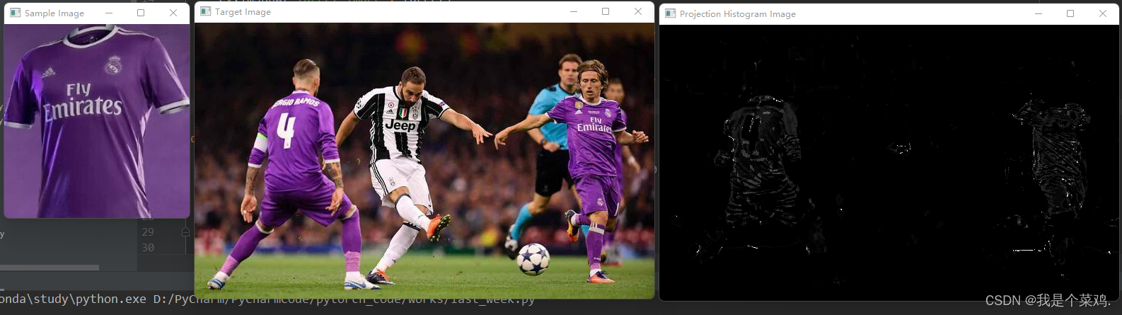
6、直方图反向映射

6.1 基本概念和作用

用直方图模型去目标图像中寻找是否有相似的对象，实现对特定对象的检测

6.2 代码示例

①加载图片；
②将图像从RGB色彩空间转换到HSV色彩空间；
③计算直方图并归一化（calcHist()、normalize()）;
④计算反向投影图像（calcBackProject() ）;


import cv2 as cv
import matplotlib.pyplot as plt
import numpy as np


def hist_projection_demo():
    target = cv.imread('../images/target.jpg', 1)
    sample = cv.imread('../images/sample_.png', 1)

    sample_hsv = cv.cvtColor(sample, cv.COLOR_BGR2HSV)
    target_hsv = cv.cvtColor(target, cv.COLOR_BGR2HSV)

    cv.imshow('Sample Image', sample)
    cv.imshow('Target Image', target)

    sampleHist = cv.calcHist([sample_hsv], [0, 1], None, [32, 48], [0, 180, 0, 256])
    cv.normalize(sampleHist, sampleHist, 0, 255, cv.NORM_MINMAX)

    dst = cv.calcBackProject([target_hsv], [0, 1], sampleHist, [0, 180, 0, 256], 1)
    cv.imshow('Projection Histogram Image', dst)


def hist2D_demo(image):
    hsv = cv.cvtColor(image, cv.COLOR_BGR2HSV)
    hist = cv.calcHist([hsv], [0, 1], None, [180, 256], [0, 180, 0, 255])

    plt.imshow(hist, interpolation='nearest')
    plt.title('Histogram 2D Image')
    plt.show()


hist_projection_demo()
cv.waitKey(0)
cv.destroyAllWindows()

在这里插入图片描述

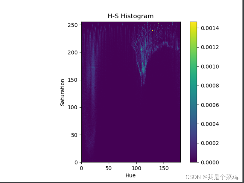
7、H-S直方图

7.1 基本概念和作用

用于表示图像颜色分布的直方图。它基于图像中每个像素的色调（Hue）和饱和度（Saturation）信息，通过统计这两个颜色属性的分布情况，形成直方图。H-S直方图是在颜色空间中对颜色特征进行可视化和分析的工具。应用于在颜色分析、图像检索和目标识别等

7.2 示例代码

import cv2
import numpy as np
import matplotlib.pyplot as plt

def compute_hs_histogram(image):
    # 将图像从BGR颜色空间转换为HSV颜色空间
    hsv_image = cv2.cvtColor(image, cv2.COLOR_BGR2HSV)

    # 提取Hue和Saturation通道
    hue_channel = hsv_image[:,:,0]
    saturation_channel = hsv_image[:,:,1]

    # 计算Hue-Saturation直方图
    hs_histogram, _, _ = np.histogram2d(hue_channel.flatten(), saturation_channel.flatten(), bins=[180, 256], range=[[0, 180], [0, 256]])

    # 归一化直方图
    hs_histogram /= hs_histogram.sum()

    return hs_histogram

# 读取图像
image = cv2.imread('../images/4.jpg')

# 计算H-S直方图
hs_histogram = compute_hs_histogram(image)

# 显示H-S直方图
plt.imshow(hs_histogram.T, cmap='viridis', extent=[0, 180, 0, 256], interpolation='nearest')
plt.title('H-S Histogram')
# 色调
plt.xlabel('Hue')
# 饱和度
plt.ylabel('Saturation')
plt.colorbar()
plt.show()

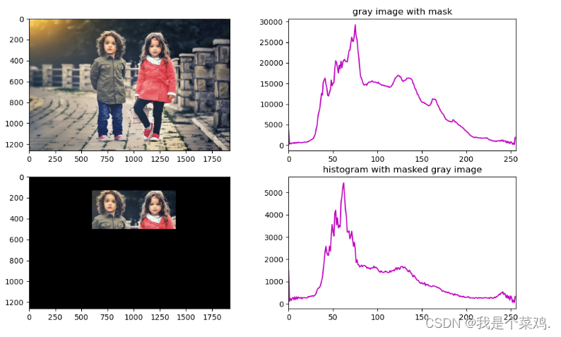
8、自定义直方图

8.1 mask

# 1 导入库
import cv2
import matplotlib.pyplot as plt
import numpy as np

# 2 方法：显示图片
def show_image(image, title, pos):
    img_RGB = image[:, :, ::-1] # BGR to RGB
    plt.title(title)
    plt.subplot(2, 2, pos)
    plt.imshow(img_RGB)

# 3 方法：显示灰度直方图
def show_histogram(hist, title, pos, color):
    plt.subplot(2, 2, pos)
    plt.title(title)
    plt.xlim([0, 256])
    plt.plot(hist, color=color)

# 4 主函数
def main():
    # 5 创建画布
    plt.figure(figsize=(12, 7))
    plt.suptitle("Gray Image and Histogram with mask", fontsize=4, fontweight="bold")

    # 6 读取图片并灰度转换，计算直方图，显示
    img_gray = cv2.imread("../images/children.jpg", cv2.COLOR_BGR2GRAY) # 读取并进行灰度转换
    img_gray_hist = cv2.calcHist([img_gray], [0], None, [256], [0, 256]) # 计算直方图
    show_image(img_gray, "image gray", 1)
    show_histogram(img_gray_hist, "image gray histogram", 2, "m")

    # 7 创建mask，计算位图，直方图
    mask = np.zeros(img_gray.shape[:2], np.uint8)
    mask[130:500, 600:1400] = 255 # 获取mask，并赋予颜色
    img_mask_hist = cv2.calcHist([img_gray], [0], mask, [256], [0, 256]) # 计算mask的直方图

    # 8 通过位运算（与预算）计算带有mask的灰度图片
    mask_img = cv2.bitwise_and(img_gray, img_gray, mask = mask)

    # 9 显示带有mask的图片和直方图
    show_image(mask_img, "gray image with mask", 3)
    show_histogram(img_mask_hist, "histogram with masked gray image", 4, "m")

    plt.show()
if __name__ == '__main__':
    main()

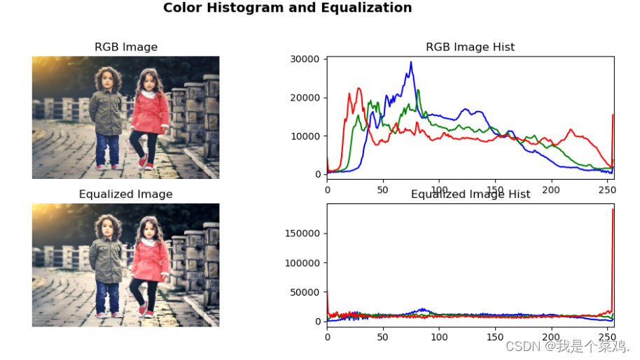
9、彩色直方图均衡

示例代码

import cv2
import matplotlib.pyplot as plt
import numpy as np

# 显示图片
def show_image(image, title, pos):
    plt.subplot(3, 2, pos)
    plt.title(title)
    image_RGB = cv2.cvtColor(image, cv2.COLOR_BGR2RGB)  # BGR to RGB
    plt.imshow(image_RGB)
    plt.axis("off")

# 显示彩色直方图 b, g, r
def show_histogram(hist, title, pos, color):
    plt.subplot(3, 2, pos)
    plt.title(title)
    plt.xlim([0, 256])
    for h, c in zip(hist, color):  # color: ('b', 'g', 'r')
        plt.plot(h, color=c)

# 计算彩色直方图
def calc_color_hist(image):
    hist = []
    hist.append(cv2.calcHist([image], [0], None, [256], [0, 256]))
    hist.append(cv2.calcHist([image], [1], None, [256], [0, 256]))
    hist.append(cv2.calcHist([image], [2], None, [256], [0, 256]))
    return hist

# 彩色直方图均衡化
def color_histogram_equalization(image):
    # 将图像从BGR颜色空间转换为YUV颜色空间
    yuv_image = cv2.cvtColor(image, cv2.COLOR_BGR2YUV)

    # 对亮度通道进行直方图均衡化
    yuv_image[:, :, 0] = cv2.equalizeHist(yuv_image[:, :, 0])

    # 将图像从YUV颜色空间转换回BGR颜色空间
    equalized_image = cv2.cvtColor(yuv_image, cv2.COLOR_YUV2BGR)

    return equalized_image

# 主函数
def main():
    # 创建画布
    plt.figure(figsize=(12, 8))
    plt.suptitle("Color Histogram and Equalization", fontsize=14, fontweight="bold")

    # 读取原图片
    img = cv2.imread("../images/children.jpg")

    # 计算原始直方图
    img_hist = calc_color_hist(img)

    # 显示原始图片和直方图
    show_image(img, "RGB Image", 1)
    show_histogram(img_hist, "RGB Image Hist", 2, ('b', 'g', 'r'))

    # 彩色直方图均衡化
    equalized_img = color_histogram_equalization(img)
    equalized_img_hist = calc_color_hist(equalized_img)

    # 显示均衡化后的图片和直方图
    show_image(equalized_img, 'Equalized Image', 3)
    show_histogram(equalized_img_hist, 'Equalized Image Hist', 4, ('b', 'g', 'r'))

    plt.show()

if __name__ == '__main__':
    main()

10、直方图变换（累计）

10.1 基本概念和作用

对图像的像素值进行累积，在直方图中，累积表示了某个像素值及其以下的像素值的总和。
累积直方图可以用以下步骤来计算：
-计算原始直方图（直方图中每个 bin 的值）。
-对原始直方图进行累加操作，得到累积直方图。

10.2 示例代码

import cv2
import matplotlib.pyplot as plt
import numpy as np


# 显示图片
def show_image(image, title, pos):
    plt.subplot(4, 2, pos)
    plt.title(title)
    image_RGB = cv2.cvtColor(image, cv2.COLOR_BGR2RGB)  # BGR to RGB
    plt.imshow(image_RGB)
    plt.axis("off")


# 显示彩色直方图 b, g, r
def show_histogram(hist, title, pos, color):
    plt.subplot(4, 2, pos)
    plt.title(title)
    plt.xlim([0, 256])
    for h, c in zip(hist, color):  # color: ('b', 'g', 'r')
        plt.plot(h, color=c)


# 计算彩色直方图
def calc_color_hist(image):
    hist = []
    hist.append(cv2.calcHist([image], [0], None, [256], [0, 256]))
    hist.append(cv2.calcHist([image], [1], None, [256], [0, 256]))
    hist.append(cv2.calcHist([image], [2], None, [256], [0, 256]))
    return hist


# 计算累积直方图
def calc_cumulative_hist(hist):
    cumulative_hist = [np.cumsum(channel_hist) for channel_hist in hist]
    return cumulative_hist


# 主函数
def main():
    # 创建画布
    plt.figure(figsize=(12, 16))
    plt.suptitle("Color Histogram, Equalization, and Cumulative Histogram", fontsize=14, fontweight="bold")

    # 读取原图片
    img = cv2.imread("../images/children.jpg")

    # 计算原始直方图
    img_hist = calc_color_hist(img)

    # 显示原始图片和直方图
    show_image(img, "RGB Image", 1)
    show_histogram(img_hist, "RGB Image Hist", 2, ('b', 'g', 'r'))

    # 计算并显示累积直方图
    cumulative_hist = calc_cumulative_hist(img_hist)
    show_histogram(cumulative_hist, 'Cumulative Histogram', 4, ('b', 'g', 'r'))

    plt.show()


if __name__ == '__main__':
    main()

11、直方图对比

11.1 基本概念和作用

比较两幅图像的直方图来评估它们相似性的方法。基本原理是比较图像的颜色或灰度分布。

11.2 示例代码

在这里插入图片描述
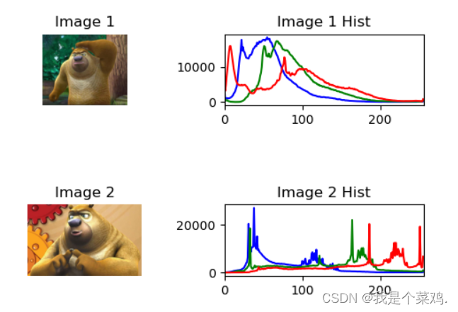
Histogram Compare Result: 0.8173332006305307

import cv2
import matplotlib.pyplot as plt
import numpy as np

# 显示图片
def show_image(image, title, pos):
    plt.subplot(4, 2, pos)
    plt.title(title)
    image_RGB = cv2.cvtColor(image, cv2.COLOR_BGR2RGB)
    plt.imshow(image_RGB)
    plt.axis("off")

# 显示彩色直方图 b, g, r
def show_histogram(hist, title, pos, color):
    plt.subplot(4, 2, pos)
    plt.title(title)
    plt.xlim([0, 256])
    for h, c in zip(hist, color):  # color: ('b', 'g', 'r')
        plt.plot(h, color=c)

# 计算彩色直方图
def calc_color_hist(image):
    hist = []
    hist.append(cv2.calcHist([image], [0], None, [256], [0, 256]))
    hist.append(cv2.calcHist([image], [1], None, [256], [0, 256]))
    hist.append(cv2.calcHist([image], [2], None, [256], [0, 256]))
    return hist



# 直方图比较
def histogram_compare(image1, image2):
    hist1 = cv2.calcHist([image1], [0, 1, 2], None, [256, 256, 256], [0, 256, 0, 256, 0, 256])
    hist2 = cv2.calcHist([image2], [0, 1, 2], None, [256, 256, 256], [0, 256, 0, 256, 0, 256])

    # 使用巴氏距离进行直方图比较
    result = cv2.compareHist(hist1, hist2, cv2.HISTCMP_BHATTACHARYYA)
    return result

# 主函数
def main():
    # 读取图片1
    img1 = cv2.imread("../images/11-1.jpg")

    # 读取图片2
    img2 = cv2.imread("../images/11-2.jpg")

    # 显示图片1
    show_image(img1, "Image 1", 1)

    # 计算并显示图片1的直方图
    img1_hist = calc_color_hist(img1)
    show_histogram(img1_hist, "Image 1 Hist", 2, ('b', 'g', 'r'))

    # 显示图片2
    show_image(img2, "Image 2", 5)

    # 计算并显示图片2的直方图
    img2_hist = calc_color_hist(img2)
    show_histogram(img2_hist, "Image 2 Hist", 6, ('b', 'g', 'r'))


    # 直方图比较
    hist_compare_result = histogram_compare(img1, img2)
    print(f"Histogram Compare Result: {hist_compare_result}")

    plt.show()

if __name__ == '__main__':
    main()