机器学习逐渐放弃：分类（一）

MNIST

hello world。。。sklearn 有很多助手可以下载流行数据集，加载的数据集通常是类似于字典的结果

• DESCR 描述数据集
• data 一个数组，每个实例一行，每个特征一列
• target 一个带有标签的数组

>>> from sklearn.datasets import fetch_openml    # 需要科学上网。。。
>>> mnist = fetch_openml('mnist_784', version=1)
>>> mnist.keys()
dict_keys(['data', 'target', 'feature_names', 'DESCR', 'details',
				 'categories', 'url'])

X, y = mnist["data"], mnist["target"]
X.shape,y.shape
((70000, 784), (70000,))
# 7万张图片，每个图片784个特征（28*28），每个特征代表一个像素

%matplotlib inline  
# 调用matplotlib.pyplot的绘图函数plot()进行绘图的时候，或者生成一个figure画布的时候，可以直接在你的python console里面生成图像。
import matplotlib as mpl
import matplotlib.pyplot as plt

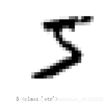
some_digit = X[0]
some_digit_image = some_digit.reshape(28, 28)
plt.imshow(some_digit_image, cmap=mpl.cm.binary)  # 二值化
plt.axis("off")
plt.show()
print(y[0],type(y[0]))   
# 标签是字符串，但我们需要数字
y = y.astype(np.uint8)

# 分出测试集和训练集，MNIST数据集已经分成训练集（前6万张图片）和测试集（最后1万张图片）了
X_train, X_test, y_train, y_test = X[:60000], X[60000:], y[:60000], y[60000:]
   
def plot_digits(instances, images_per_row=10, **options):
    size = 28
    images_per_row = min(len(instances), images_per_row)
    images = [instance.reshape(size,size) for instance in instances]
    n_rows = (len(instances) - 1) // images_per_row + 1  # 好强啊，这就是大佬吗
    row_images = []
    n_empty = n_rows * images_per_row - len(instances)    # 太细节了吧
    images.append(np.zeros((size, size * n_empty)))  
    for row in range(n_rows):
        rimages = images[row * images_per_row : (row + 1) * images_per_row]
        row_images.append(np.concatenate(rimages, axis=1))   # 将每个图拼成一个大图
    image = np.concatenate(row_images, axis=0)
    plt.imshow(image, cmap = mpl.cm.binary, **options)
    plt.axis("off")
    
plt.figure(figsize=(9,9))
example_images = X[:99]
plot_digits(example_images, images_per_row=10)   # 感觉就这一个函数就有好多可以开发的想法。。

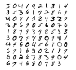
可以看到数据是经过混洗的，保证交叉验证时所有的折叠都差不多，此外有些算法对训练实例的顺序敏感，如果连续输入许多相似的实例，可能导致执行性能不佳。

训练二元分类器

尝试识别一个数字，就是分类两个类别

# 为分类任务创建目标向量
y_train_5 = (y_train == 5)   # bool
y_test_5 = (y_test == 5)

# 挑选一个分类器开始训练，比如SGD 随机梯度下降，这个可以有效的处理大型数据集
from sklearn.linear_model import SGDClassifier
sgd_clf = SGDClassifier(max_iter = 1000, tol=le-3, random_state=42)
sgd_clf.fit(X_train,y_train_5) # SGD的训练时随机的，random_state 参数可以让结果复现
SGDClassifier(random_state=42)   

sgd_clf.predict([X[0]])        # 预测一下
array([ True])

性能测量

评估分离器比评估回归器要难很多。

使用交叉验证测量准确率

from sklearn.model_selection import cross_val_scroe  # 3 折交叉验证
cross_val_score(sgd_clf,X_train,y_train_5,cv=3,scoring = 'accuarcy')
array([0.95035, 0.96035, 0.9604 ])   # 挺耗时间的，，，，

from sklearn.model_selection import StratifiedKFold    # k 折交叉验证的实现方法
from sklearn.base import clone
# 分层抽样
skfolds = StratifiedKFold(n_splits=3, shuffle=True, random_state=42)
for train_index, test_index in skfolds.split(X_train, y_train_5):
    clone_clf = clone(sgd_clf)   
    # 克隆一个新的估算器，对模型的深度复制，产生的估算器是没有在数据上拟合过的。
    X_train_folds = X_train[train_index]
    y_train_folds = y_train_5[train_index]
    X_test_fold = X_train[test_index]
    y_test_fold = y_train_5[test_index]

    clone_clf.fit(X_train_folds, y_train_folds)
    y_pred = clone_clf.predict(X_test_fold)
    n_correct = sum(y_pred == y_test_fold)  # 统计正确的次数
    print(n_correct / len(y_pred))
0.9669
0.91625      # 正确率类似的
0.96785

from sklearn.base import BaseEstimator
class Never5Classifier(BaseEstimator):    # 这就是只预测为 非5
    def fit(self,X,y=None):
        pass
    def predict(self,X):
        return np.zeros((len(X),1),dtype=bool)
never_5_clf = Never5Classifier()
cross_val_score(never_5_clf,X_train,y_train_5,cv=3,scoring='accuracy')
>>>array([0.91125, 0.90855, 0.90915])   # 正确率也不低


# 说明正确率对分类来说不是首要性能指标，特别是处理有偏数据时。

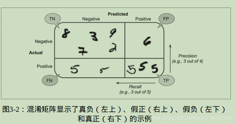
混淆矩阵

就是统计 A 类被实例错误分成 B 类的次数。

from sklearn.model_selection import cross_val_predict   
y_train_pred = cross_val_predict(sgd_clf, X_train, y_train_5, cv=3)
'''
这个函数也是执行k 折交叉验证，但返回的时每个折 的预测。对每个实例都可以得到一个干净的预测
就是模型预测时使用的数据在训练期间没有出现。
'''
from sklearn.metrics import confusion_matrix    # 构建混淆矩阵
confusion_matrix(y_train_5, y_train_pred)
array([[53892,   687],
       [ 1891,  3530]])     # 完美的分类器 只会有 TP FN 两个

# 查准率 和召回率 和F1 值
from sklearn.metrics import precision_score,recall_score
precision_score(y_train_5, y_train_pred)
>>> 0.8370879772350012            # 正确率时83% ，而且只有 65% 的数字5被检测出来
recall_score(y_train_5,y_train_pred)
>>>0.6511713705958311

from sklearn.metrics import f1_score
f1_score(y_train_5,y_train_pred)
>>>0.7325171197343846

'''
 查准率和召回率是相对的，无法两个都高（精度/召回率权衡），但是可以更加看重其中之一（西瓜书中有个 Fβ来着）
 在精度/召回率权衡中，图像按照分类器的评分排名，然后取一个阈值，高于的就是正类
 这个阈值越高，召回率越低，但是查准率高
 sklearn 中，不能直接设置举止，但是可以访问它用于预测的决策分数。decision_funciton() 方法。
 返回每个实例的分数，然后就可以根据这些分数使用任意阈值进行预测。
'''
y_scores = sgd_clf.decision_function([some_digit])
y_scores
array([2164.22030239])

# 使用 cross_val_predict() 函数获取训练集中所有实例的决策分数，
y_scores = coss_val_predict(sgd_slf,X_train,y_train_5,cv=3,method="decision_function")

# 有了决策分数就可以使用这个计算所有可能阈值的查准率和召回率
from sklearn.metrics import precision_recall_curve    
precisions, recalls, thresholds = precision_recall_curve(y_train_5, y_scores)

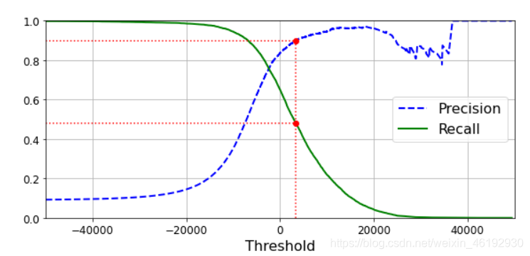
# 绘制一下不同阈值对应的查准率和召回率
def plot_precision_recall_vs_threshold(precisions, recalls, thresholds):
    plt.plot(thresholds, precisions[:-1], "b--", label="Precision", linewidth=2)
    plt.plot(thresholds, recalls[:-1], "g-", label="Recall", linewidth=2)
    plt.legend(loc="center right", fontsize=16)
    plt.xlabel("Threshold", fontsize=16)        
    plt.grid(True)                              
    plt.axis([-50000, 50000, 0, 1])            

recall_90_precision = recalls[np.argmax(precisions >= 0.90)]  # # 查准率为90 的时候对应的召回率和阈值
threshold_90_precision = thresholds[np.argmax(precisions >= 0.90)]


plt.figure(figsize=(8, 4))                                                                  
plot_precision_recall_vs_threshold(precisions, recalls, thresholds)
plt.plot([threshold_90_precision, threshold_90_precision], [0., 0.9], "r:")                
plt.plot([-50000, threshold_90_precision], [0.9, 0.9], "r:")                                
plt.plot([-50000, threshold_90_precision], [recall_90_precision, recall_90_precision], "r:")
plt.plot([threshold_90_precision], [0.9], "ro")                                           
plt.plot([threshold_90_precision], [recall_90_precision], "ro")                            
save_fig("precision_recall_vs_threshold_plot")                                            
plt.show()
'''
提高阈值查准率有可能是下降的（总体是上升的），另外阈值上升召回率下降，召回率的曲线就很平滑。
'''

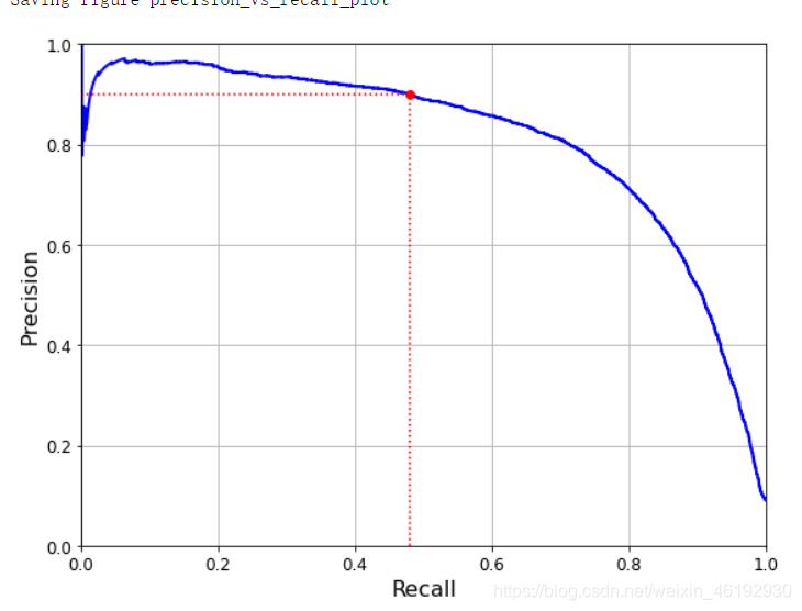
还有就是 PR 曲线，

def plot_precision_vs_recall(precisions, recalls):
    plt.plot(recalls, precisions, "b-", linewidth=2)
    plt.xlabel("Recall", fontsize=16)
    plt.ylabel("Precision", fontsize=16)
    plt.axis([0, 1, 0, 1])
    plt.grid(True)

plt.figure(figsize=(8, 6))
plot_precision_vs_recall(precisions, recalls)
plt.plot([recall_90_precision, recall_90_precision], [0., 0.9], "r:")
plt.plot([0.0, recall_90_precision], [0.9, 0.9], "r:")
plt.plot([recall_90_precision], [0.9], "ro")
save_fig("precision_vs_recall_plot")
plt.show()

threshold_90_precision = thresholds[np.argmax(precisions >= 0.90)]
print(threshold_90_precision)
y_train_pred_90 = (y_scores >= threshold_90_precision)
print(precision_score(y_train_5, y_train_pred_90),
     recall_score(y_train_5, y_train_pred_90))
3370.0194991439557
0.9000345901072293 0.4799852425751706     # 精度很高召回率就低了。。

ROC 曲线

绘制的时真正例率（TNR， 就是召回率，灵敏度) 和假正例率（FPR，被错误分类为正类的负类实例比率 ，等于1-TNR（被正确分类为负类的负类实例比率）），

from sklearn.metrics import roc_curve  # 计算多种阈值的TPR FPR

fpr, tpr, thresholds = roc_curve(y_train_5, y_scores) # 样本分类标签，每个样本的预测结果，pos_label指定正标签
# 根据每一个阈值判断 scores，小于阈值就是负样本，来计算FPR TPR
# thresholds 是从低值到高值排序的，需要反转对应FPR TPR

def plot_roc_curve(fpr, tpr, label=None):
    plt.plot(fpr, tpr, linewidth=2, label=label)
    plt.plot([0, 1], [0, 1], 'k--') 
    plt.axis([0, 1, 0, 1])                                    
    plt.xlabel('False Positive Rate (Fall-Out)', fontsize=16) 
    plt.ylabel('True Positive Rate (Recall)', fontsize=16)    
    plt.grid(True)                                            

plt.figure(figsize=(8, 6))                                    
plot_roc_curve(fpr, tpr)
fpr_90 = fpr[np.argmax(tpr >= recall_90_precision)]           
plt.plot([fpr_90, fpr_90], [0., recall_90_precision], "g:")   
plt.plot([0.0, fpr_90], [recall_90_precision, recall_9
0_precision], "r:")  
plt.plot([fpr_90], [recall_90_precision], "ro")                                                   
plt.show()

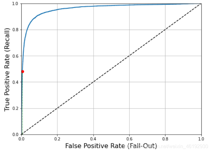
AUC 就是ROC 下的面积，完美的分类器AUC = 1，纯随机分类器AUC 等于0.5，
ROC 与 PR 的选择：正类少或更关注假正类而不是假负类，选择PR，

>>> from sklearn.metrics import roc_auc_score
>>> roc_auc_score(y_train_5, y_scores)      # SGD 的AUC
0.9611778893101814

from sklearn.ensemble import RandomForestClassifier
forest_clf = RandomForestClassifier(n_estimators=100, random_state=42)
y_probas_forest = cross_val_predict(forest_clf, X_train, y_train_5, cv=3,
                                    method="predict_proba")
'''
获取训练集中每个实例的分数，随机森林分类器类没有decision_function() 方法
而是有 dict_proba() 方法，返回一个数组，每行代表一个实例，每列代表一个类别
就是某个给定实例属于某个给定类别的概率
'''
y_probas_forest[:2],y_probas_forest.shape
(array([[0.11, 0.89],
        [0.99, 0.01]]),
 (60000, 2))
 
y_scores_forest = y_probas_forest[:, 1]      # 需要标签和分数，但我们提供的是正类概率
fpr_forest, tpr_forest, thresholds_forest = roc_curve(y_train_5,y_scores_forest)

recall_for_forest = tpr_forest[np.argmax(fpr_forest >= fpr_90)]

plt.figure(figsize=(8, 6))
plt.plot(fpr, tpr, "b:", linewidth=2, label="SGD")
plot_roc_curve(fpr_forest, tpr_forest, "Random Forest")
plt.plot([fpr_90, fpr_90], [0., recall_90_precision], "r:")
plt.plot([0.0, fpr_90], [recall_90_precision, recall_90_precision], "r:")
plt.plot([fpr_90], [recall_90_precision], "ro")
plt.plot([fpr_90, fpr_90], [0., recall_for_forest], "r:")
plt.plot([fpr_90], [recall_for_forest], "ro")
plt.grid(True)
plt.legend(loc="lower right", fontsize=16)
plt.show()

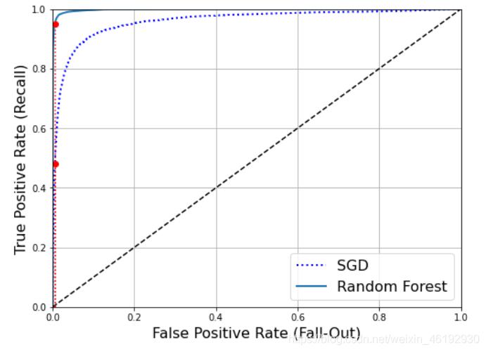
roc_auc_score(y_train_5, y_scores_forest)    # 随机森林的AUC
0.9983436731328145    # 很接近1 了

y_train_pred_forest = cross_val_predict(forest_clf, X_train, y_train_5, cv=3)
precision_score(y_train_5, y_train_pred_forest)   # 看看查准率和召回率
0.9905083315756169
recall_score(y_train_5, y_train_pred_forest)
0.8662608374838591

多分类

OVO 策略，一对一，就是训练多个二元分类器（N个类别两两搭配），然后看结果中那个类最多。优势是每个分类器只需要用到部分训练集对其必须区分的两个类进行训练

OVR 策略，一对剩余，就是对一个类和剩余类进行分类，对每个分类器的决策分数取最高的那个。

MVM 策略，纠错输出码啥的。。

sklearn 可以检测你尝试使用二元分类法进行多分类任务，然后自动选择OVR OVO，掉包真香。

from sklearn.svm import SVC

svm_clf = SVC(gamma="auto", random_state=42) # 使用类0-9 进行训练然后预测
svm_clf.fit(X_train[:1000], y_train[:1000]) # y_train, not y_train_5
svm_clf.predict([some_digit])    # 这里实际训练了45个二元分类器，获取决策分数选最高的类。
array([5], dtype=uint8)         # 预测正确

some_digit_scores = svm_clf.decision_function([some_digit])
some_digit_scores  # 十个分数，每个类一个，5的得分最高
array([[ 2.81585438,  7.09167958,  3.82972099,  0.79365551,  5.8885703 ,
         9.29718395,  1.79862509,  8.10392157, -0.228207  ,  4.83753243]])
>>> np.argmax(some_digit_scores)
5
>>> svm_clf.classes_      # 目标类的列表会存储在class_属性中，按值得大小排序，这里每个类得索引对应类本身。
array([0, 1, 2, 3, 4, 5, 6, 7, 8, 9], dtype=uint8)
>>> svm_clf.classes_[5]
5

# 强制使用 OVO 或 OVR 策略，可以使用OneVsOneClassifier或OneVsRestClassifier类
# 需要构建一个实例，然后将分类器传给构造函数（可以不是二元分类器）
from sklearn.multiclass import OneVsRestClassifier
ovr_clf = OneVsRestClassifier(SVC(gamma="auto", random_state=42))
ovr_clf.fit(X_train[:1000], y_train[:1000])
ovr_clf.predict([some_digit]),len(ovr_clf.estimators_)  # 类得个数吧
(array([5], dtype=uint8), 10)


sgd_clf.fit(X_train, y_train)
sgd_clf.predict([some_digit])  # SGD分类器直接可以将实例分为多个类，就不用OVR OVO
array([3], dtype=uint8)   # 尴尬，，预测错了。。。

sgd_clf.decision_function([some_digit])  
# 这个函数可以获得分类器将每个实例分类为每个类得概率
array([[-31893.03095419, -34419.69069632,  -9530.63950739,    # 确实第四个分数最高。。
          1823.73154031, -22320.14822878,  -1385.80478895,
        -26188.91070951, -16147.51323997,  -4604.35491274,
        -12050.767298  ]])

cross_val_score(sgd_clf, X_train, y_train, cv=3, scoring="accuracy")
# 使用交叉验证来评估这个分类器，正确率还是可以得
array([0.87365, 0.85835, 0.8689 ])

from sklearn.preprocessing import StandardScaler
scaler = StandardScaler()        # 进行简单缩放就可以将准确率提高接近90
X_train_scaled = scaler.fit_transform(X_train.astype(np.float64))
cross_val_score(sgd_clf, X_train_scaled, y_train, cv=3, scoring="accuracy")
array([0.8983, 0.891 , 0.9018])