3-5 特征离散化

3.5 特征离散化

请参考《数据准备和特征工程》中的相关章节，调试如下代码。

---

本节的视频课程：特征离散化

3.5.1 无监督离散化

基础知识

import pandas as pd

ages = pd.DataFrame({'years':[10, 14, 30, 53, 67, 32, 45], 
                    'name':['A', 'B', 'C', 'D', 'E', 'F', 'G']})
ages

	years	name
0	10	A
1	14	B
2	30	C
3	53	D
4	67	E
5	32	F
6	45	G

# 将‘years’划分为3个等宽的区间
pd.cut(ages['years'],3)

0    (9.943, 29.0]
1    (9.943, 29.0]
2     (29.0, 48.0]
3     (48.0, 67.0]
4     (48.0, 67.0]
5     (29.0, 48.0]
6     (29.0, 48.0]
Name: years, dtype: category
Categories (3, interval[float64]): [(9.943, 29.0] < (29.0, 48.0] < (48.0, 67.0]]

pd.qcut(ages['years'],3)

0    (9.999, 30.0]
1    (9.999, 30.0]
2    (9.999, 30.0]
3     (45.0, 67.0]
4     (45.0, 67.0]
5     (30.0, 45.0]
6     (30.0, 45.0]
Name: years, dtype: category
Categories (3, interval[float64]): [(9.999, 30.0] < (30.0, 45.0] < (45.0, 67.0]]

# labels=[0, 1, 2]将离散化的三个区间分别用0，1，2代替
klass = pd.cut(ages['years'], 3, labels=[0, 1, 2])    

ages['label'] = klass
ages

	years	name	label
0	10	A	0
1	14	B	0
2	30	C	1
3	53	D	2
4	67	E	2
5	32	F	1
6	45	G	1

ages2 = pd.DataFrame({'years':[10, 14, 30, 53, 300, 32, 45], 
                      'name':['A', 'B', 'C', 'D', 'E', 'F', 'G']})

klass2 = pd.cut(ages2['years'], 3, labels=['Young', 'Middle', 'Senior'])    # ②
ages2['label'] = klass2
ages2

	years	name	label
0	10	A	Young
1	14	B	Young
2	30	C	Young
3	53	D	Young
4	300	E	Senior
5	32	F	Young
6	45	G	Young

ages2 = pd.DataFrame({'years':[10, 14, 30, 53, 300, 32, 45],
                      'name':['A', 'B', 'C', 'D', 'E', 'F', 'G']})

# bins既可以表示划分的区间个数，也可以表示划分区间的分割点
klass2 = pd.cut(ages2['years'], bins=[9, 30, 50, 300], labels=['Young', 'Middle', 'Senior']) 
  
ages2['label'] = klass2
ages2

	years	name	label
0	10	A	Young
1	14	B	Young
2	30	C	Young
3	53	D	Senior
4	300	E	Senior
5	32	F	Middle
6	45	G	Middle

from sklearn.preprocessing import KBinsDiscretizer

# encode='ordinal'：离散化之后，以整数数值标记相应的记录
# 还可选择onehot：离散化之后在进行onehot编码，并且返回稀疏数组。
# onehot-dense：离散化之后在进行onehot编码，并且返回数组。

# strategy='uniform':离散化后每个分区宽度相同
# quantile：默认值，每个分区样本数相同
# kmeans：根据k-means聚类算法设置分区

kbd = KBinsDiscretizer(n_bins=3, encode='ordinal', strategy='uniform')   

trans = kbd.fit_transform(ages[['years']])    
ages['kbd'] = trans[:, 0]    
ages

	years	name	label	kbd
0	10	A	0	0.0
1	14	B	0	0.0
2	30	C	1	1.0
3	53	D	2	2.0
4	67	E	2	2.0
5	32	F	1	1.0
6	45	G	1	1.0

项目案例

import numpy as np 
from sklearn.datasets import load_iris
from sklearn.preprocessing import KBinsDiscretizer
from sklearn.tree import DecisionTreeClassifier
from sklearn.model_selection import cross_val_score

iris = load_iris()
iris.feature_names

['sepal length (cm)',
 'sepal width (cm)',
 'petal length (cm)',
 'petal width (cm)']

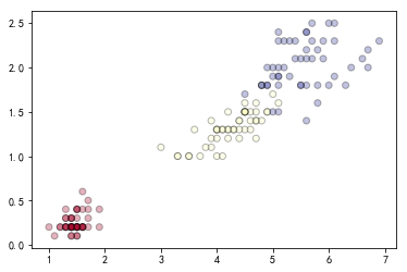
# 选择2，3两列的数据
X = iris.data[:, [2, 3]]

%matplotlib inline
import matplotlib.pyplot as plt


# 绘制未离散化的散点图
# c=y：表示的是色彩或颜色序列，可选，默认蓝色’b’。c可以是一个RGB或RGBA二维行数组。
# cmap：标量或者是一个colormap的名字。为c中的target一一上色。

y = iris.target
plt.scatter(X[:, 0], X[:, 1], c=y, alpha=0.3,  cmap=plt.cm.RdYlBu, edgecolor='black')

# 绘制uniform离散化策略后的散点图
Xd = KBinsDiscretizer(n_bins=10, encode='ordinal', strategy='uniform').fit_transform(X)

plt.scatter(Xd[:, 0], Xd[:, 1], c=y, cmap=plt.cm.RdYlBu, edgecolor='black')

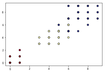
# 构建决策树模型，用于评估离散化后的效果
dtc = DecisionTreeClassifier(random_state=0)    

# score1为未离散化的评估得分，cv：可迭代的次数
score1 = cross_val_score(dtc, X, y, cv=5)    
score2 = cross_val_score(dtc, Xd, y, cv=5)    

print('未离散化平均值：', '%.3f'%np.mean(score1), '未离散化标准差：', '%.3f'%np.std(score1))
print('离散化后平均值：', '%.3f'%np.mean(score2), '离散化后标准差：', '%.3f'%np.std(score2))

未离散化平均值： 0.947 未离散化标准差： 0.040
离散化后平均值： 0.960 离散化后标准差： 0.033

# kmeans离散化策略
km = KBinsDiscretizer(n_bins=3, encode='ordinal', strategy='kmeans').fit_transform(X)    

score3 = cross_val_score(dtc, km, y, cv=5)
print('kmeans离散化后平均值：', '%.3f'%np.mean(score3), 'kmeans离散化后标准差：', '%.3f'%np.std(score3))

kmeans离散化后平均值： 0.973 kmeans离散化后标准差： 0.025

动手练习

import numpy as np

# 定义一个随机数种子
rnd = np.random.RandomState(42)

# 产生一个100个元素的数组，其中每个元素都是在[-3,3]区间内均匀分布的随机数
X = rnd.uniform(-3, 3, size=100)

y = np.sin(X) + rnd.normal(size=len(X)) / 3
X = X.reshape(-1, 1)
X

array([[-0.75275929],
       [ 2.70428584],
       [ 1.39196365],
		.....
       [-0.43475389],
       [-2.84748524],
       [-2.35265144]])

# 复制文件到matplotlib字体路径
!cp simhei.ttf /opt/conda/envs/python35-paddle120-env/lib/python3.7/site-packages/matplotlib/mpl-data/fonts/ttf/
# 删除matplotlib的缓冲目录
!rm -rf .cache/matplotlib
# 重启内核

%matplotlib inline
import numpy as np
import matplotlib.pyplot as plt

from sklearn.linear_model import LinearRegression
from sklearn.preprocessing import KBinsDiscretizer
from sklearn.tree import DecisionTreeRegressor

# 设置显示中文
plt.rcParams['font.sans-serif'] = ['SimHei'] # 指定默认字体
plt.rcParams['axes.unicode_minus'] = False   # 解决保存图像是负号'-'显示为方块的问题

# onehot编码，默认区间等宽离散化
kbd = KBinsDiscretizer(n_bins=10, encode='onehot')
X_binned = kbd.fit_transform(X)

# ncols=2：创建一行两个子图
# sharey=True：所有子图共享 y 轴
# figsize=(10, 4)：设置子图大小为10*4
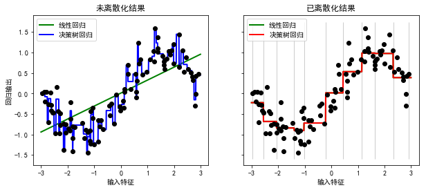
fig, (ax1, ax2) = plt.subplots(ncols=2, sharey=True, figsize=(10, 4))

# 生成一个指定大小，指定数据区间的均匀分布序列
# start：序列中数据的下界。
# end：序列中数据的上界。
# num：生成序列包含num个元素；其值默认为50。
# endpoint：取True时，序列包含最大值end；否则不包含；其值默认为True。
line = np.linspace(-3, 3, 1000, endpoint=False).reshape(-1, 1)

# 利用线性回归模型对原始数据进行预测
lreg = LinearRegression().fit(X, y)

ax1.plot(line, lreg.predict(line), 
         linewidth=2, color='green', label='线性回归')

# 利用决策树回归模型对原始数据进行预测
dreg = DecisionTreeRegressor(min_samples_split=3, random_state=0).fit(X, y)
ax1.plot(line, dreg.predict(line), 
         linewidth=2, color='blue', label="决策树回归")

ax1.plot(X[:, 0], y, 'o', c='k')
ax1.legend(loc='best')
ax1.set_ylabel("回归输出")
ax1.set_xlabel("输入特征")
ax1.set_title("未离散化结果")



# 对离散化之后的数据进行预测
line_binned = kbd.transform(line)

lreg_binned = LinearRegression().fit(X_binned, y)
ax2.plot(line, lreg_binned.predict(line_binned), 
         linewidth=2, color='green', 
         linestyle='-', label='线性回归')

dreg_binned = DecisionTreeRegressor(min_samples_split=3, random_state=0).fit(X_binned, y)
ax2.plot(line, dreg_binned.predict(line_binned), 
         linewidth=2, color='red', 
         linestyle='-', label="决策树回归")

ax2.plot(X[:, 0], y, 'o', c='k')
ax2.vlines(kbd.bin_edges_[0], *plt.gca().get_ylim(), linewidth=1, alpha=0.2)
ax2.legend(loc='best')
ax2.set_xlabel("输入特征")
ax2.set_title("已离散化结果")

Text(0.5,1,'已离散化结果')

3.5.2 有监督离散化

基础知识

!mkdir /home/aistudio/external-libraries
!pip install -i https://pypi.tuna.tsinghua.edu.cn/simple entropy-based-binning -t /home/aistudio/external-libraries

import sys
sys.path.append('/home/aistudio/external-libraries')

# ebb.bin_array?

import entropy_based_binning as ebb

A = np.array([[1,1,2,3,3], [1,1,0,1,0]])

# 基于熵（信息增益）的离散化方法
# nbins=2，可划分的区间个数为2
# axis=1，以1为离散化的分割点
ebb.bin_array(A, nbins=2, axis=1)

array([[0, 0, 1, 1, 1],
       [1, 1, 0, 1, 0]])

项目案例

!pip install -i https://pypi.tuna.tsinghua.edu.cn/simple mdlp-discretization -t /home/aistudio/external-libraries

from mdlp.discretization import MDLP
from sklearn.datasets import load_iris

# 基于最小描述长度的离散化方法
transformer = MDLP()

iris = load_iris()
X, y = iris.data, iris.target
X_disc = transformer.fit_transform(X, y)
X_disc

array([[0, 1, 0, 0],
       [0, 0, 0, 0],
       [0, 1, 0, 0],
		.....
       [2, 0, 2, 2],
       [1, 1, 2, 2],
       [1, 0, 2, 2]])