图神经网络——GAT学习

1、为啥要引入GAT呢（个人理解）?

1、传统的图卷积网络（GCN）使用的是预先定义好的邻接矩阵，这也就是说明了每个节点对中心节点的影响都是固定的，无法根据邻接节点不同的特征来确定不同的依赖性。例如，你有100个朋友，其中99个都是你读研之后交到的有钱人，彼此相互联系（从这些复杂交错的联系中多多少少也能够推断出你也是一个有钱人），另一个只是你小时候的发小，只是单独的一个节点，从发小这个节点并不能推断出你是有钱人还是贫穷。 所以引入了GAT，根据节点的特征来计算出邻接权重，故能够更加清晰地标记出不同节点之间的关系。

2、GAT其中的几个重要公式：

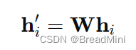
1、节点特征的线性变换：

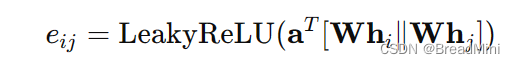
2、计算注意力系数：

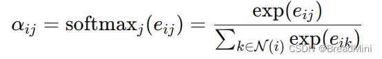
3、应用SoftMax：

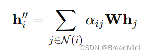
4、节点特征的聚合：

3、代码实现：

import torch
import torch.nn as nn
import torch.nn.functional as F

class GATLayer(nn.Module):
    def __init__(self, in_features, out_features, dropout, alpha, concat=True):
        super(GATLayer, self).__init__()
        self.in_features = in_features
        self.out_features = out_features
        self.dropout = dropout
        self.alpha = alpha
        self.concat = concat

        # 定义可训练的参数 W 和 a
        self.W = nn.Parameter(torch.empty(size=(in_features, out_features)))
        nn.init.xavier_uniform_(self.W.data, gain=1.414)
        self.a = nn.Parameter(torch.empty(size=(2 * out_features, 1)))
        nn.init.xavier_uniform_(self.a.data, gain=1.414)

        # 定义 LeakyReLU 激活函数
        self.leakyrelu = nn.LeakyReLU(self.alpha)

    def forward(self, h, adj):
        # 线性变换
        Wh = torch.mm(h, self.W)  # h.shape: (N, in_features), Wh.shape: (N, out_features)
        
        N = Wh.size()[0]

        # 创建多头注意力机制的输入张量
        a_input = torch.cat([Wh.repeat(1, N).view(N * N, -1), Wh.repeat(N, 1)], dim=1).view(N, -1, 2 * self.out_features)
        
        # 计算注意力系数
        e = self.leakyrelu(torch.matmul(a_input, self.a).squeeze(2))
        
        # 只保留邻接矩阵中的连接
        zero_vec = -9e15 * torch.ones_like(e)
        attention = torch.where(adj > 0, e, zero_vec)
        
        # softmax 归一化
        attention = F.softmax(attention, dim=1)
        
        # dropout
        attention = F.dropout(attention, self.dropout, training=self.training)
        
        # 聚合节点特征
        h_prime = torch.matmul(attention, Wh)
        
        if self.concat:
            return F.elu(h_prime)
        else:
            return h_prime

class GAT(nn.Module):
    def __init__(self, nfeat, nhid, nclass, dropout, alpha, nheads):
        """Dense version of GAT."""
        super(GAT, self).__init__()
        self.dropout = dropout

        # 定义多头注意力层
        self.attentions = [GATLayer(nfeat, nhid, dropout=dropout, alpha=alpha, concat=True) for _ in range(nheads)]
        for i, attention in enumerate(self.attentions):
            self.add_module('attention_{}'.format(i), attention)

        # 输出层
        self.out_att = GATLayer(nhid * nheads, nclass, dropout=dropout, alpha=alpha, concat=False)

    def forward(self, x, adj):
        x = F.dropout(x, self.dropout, training=self.training)
        x = torch.cat([att(x, adj) for att in self.attentions], dim=1)
        x = F.dropout(x, self.dropout, training=self.training)
        x = self.out_att(x, adj)
        return F.log_softmax(x, dim=1)

# 创建一个简单的图用于测试
in_features = 5
out_features = 2
nb_nodes = 3
dropout = 0.5
alpha = 0.2
nheads = 3

# 输入特征
input = torch.rand(nb_nodes, in_features)
# 邻接矩阵
adj = torch.tensor([[1, 1, 0], [1, 1, 1], [0, 1, 1]], dtype=torch.float)

# 创建模型并执行前向传播
model = GAT(in_features, out_features, nb_nodes, dropout, alpha, nheads)
output = model(input, adj)
print(output)

让我们来研究这些代码以及公式：
1、

对应代码中的： Wh = torch.mm(h, self.W)
作用：将input(35)矩阵 转变为 （32）的矩阵。

2、

对应代码中的： 创建多头注意力机制的输入张量
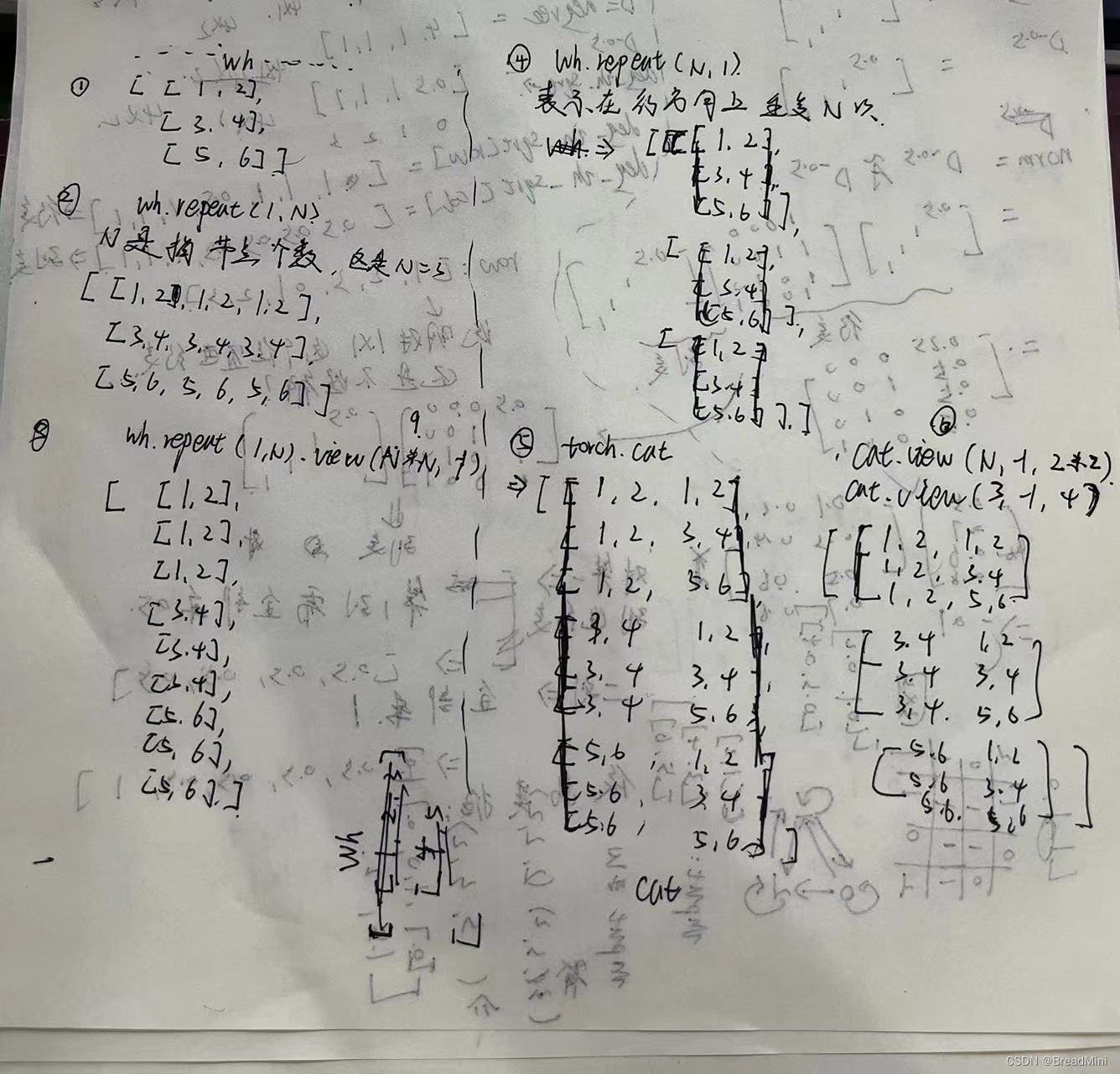
a_input = torch.cat([Wh.repeat(1, N).view(N * N, -1), Wh.repeat(N, 1)], dim=1).view(N, -1, 2 * self.out_features)
如何理解这一部分代码呢？
由步骤1 我们可以得到 Wh是（3*2） 的矩阵。

从这些运算步骤可得到结果是右下角那个。
那为啥是要这么计算呢？
理由其实很简单：看图片右下角其中一个
[1,2,1,2，
1,2,3,4，
1,2,5,6]
思考这个矩阵像啥?? [1,2],[3,4],[5,6]分别代表什么？
那不就是代表的是每个节点吗？
[1,2] 到 [1,2] 表示自环
[1,2] 到 [3,4] 表示一个节点到另一个节点。
所以 经过计算之后，能够得到每个节点到其他节点。
然后进行计算注意力系数即可。

     计算注意力系数
    e = self.leakyrelu(torch.matmul(a_input, self.a).squeeze(2))  
    这里的a_input 就是上图右下角那个张量。a 是我们自己定义的。
    a_input 是(3,3,4) 而a 是（4，1）
    计算之后得到 e 是（3，3，1）
    再使用squeeze(2) 去除第二维度的1 
    => e 是（3,3）

3、得到注意力系数attentiuon之后，进行更新h
也称之为：
聚合节点特征
h_prime = torch.matmul(attention, Wh)
attention 是（3*3），而Wh是（3 2），h_prime 是（3 2） 这样就完成了一次邻接节点特征的聚合了。

补充：
对于代码中的：
zero_vec = -9e15 * torch.ones_like(e)
attention = torch.where(adj > 0, e, zero_vec)
解释：因为可能只有 v1 到 v2，而没有v2到v1 ，所有在邻接矩阵中就体现为1 ，则保留原先数据，否则替代为一个很小的数值，减少影响。