【图神经网络——GATv2】

GATV2

GATV2 ？ 什么是GATV2呢？ 相比较于GAT 有什么区别呢？
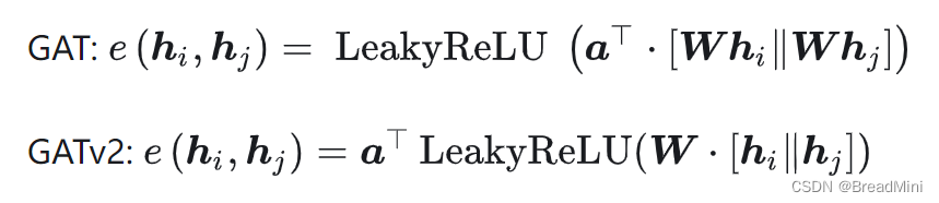
GAT：使用的是固定的注意力机制，就是说给定的节点对，其注意力系数只由其特征通过一个固定的线性变换和leakyRelu激活函数得到。
每个节点呢，都只关系自己的邻接节点，注意力系数的评分并不会受到查询节点的影响，无论是哪个查询节点，评分排名都是一样高的。
怎么理解呢？就是说：例如有1，2，3，4号人物，他们互相认识，或者不认识（也就是有没有邻接的关系），但是1号，对2，3，4号的注意力系数评分都是排名第一，并不会因为他们的邻接关系的变化而变化。

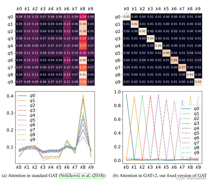
GATV2：使用的是动态的注意力机制，就是说不仅依赖于节点特征，还依赖于邻接关系。
这个”依赖于邻接关系“是不是有点难以理解呢？
似乎上一篇文章讲述到的GAT好像也依赖于邻接关系？
个人理解：对于GAT网络层来说，权重 W 一开始就是被我们所设定好的，如下面两行代码，已经是固定的了。

 self.W = nn.Parameter(torch.zeros(size=(in_features, out_features)))
        nn.init.xavier_uniform_(self.W.data, gain=1.414)

所以呢，例如其中某个节点的权重非常大，就会导致所有查询节点对该节点有所偏好，喜欢上了这个节点，所以导致每次计算出来的注意力系数评分都会比其他关键节点大大大。
而对于”GATV2“来说呢，我们并没有预先设定好权重，所以只有在运行过程中，进行计算权重，按照某种关系（邻接）进行计算权重，就去除了”静态注意力中注意力系数评分不依赖查询节点“ 这种弊端了。
注意力系数计算修改如下：

GATV2代码实现：

class GATv2Layer(nn.Module):
    def __init__(self, in_features, out_features, alpha):
        super(GATv2Layer, self).__init__()
        self.W = nn.Linear(2 * in_features, out_features)  # 线性变换
        self.a = nn.Parameter(torch.zeros(size=(out_features, 1)))
        nn.init.xavier_uniform_(self.a.data, gain=1.414)
        
        self.leakyrelu = nn.LeakyReLU(alpha)

    def forward(self, h, adj):
        N = h.size(0)
        a_input = torch.cat([h.repeat(1, N).view(N * N, -1), 
                             h.repeat(N, 1)], dim=1).view(N, -1, 2 * h.size(1))
        Wh = self.W(a_input)  # 对连接后的特征进行线性变换
        e = self.leakyrelu(torch.matmul(Wh, self.a).squeeze(2))
        zero_vec = -9e15 * torch.ones_like(e)
        attention = torch.where(adj > 0, e, zero_vec)
        attention = F.softmax(attention, dim=1)
        h_prime = torch.matmul(attention, torch.mm(h, self.W.weight.T))
        return h_prime

区别其实不咋大。

GATV2在MUTAG数据集上的应用：

任务：推断分子是否抑制HIV病毒复制

最后转换为了二分类问题

# 任务：推断分子是否抑制HIV病毒复制
import time

import torch
from torch_geometric.datasets import TUDataset
# 绘图工具
import matplotlib.pyplot as plt
import networkx as nx
# 数据加载
from torch_geometric.loader import DataLoader
import torch.nn as nn
import torch.nn.functional as F
from torch_geometric.nn import GATv2Conv
from torch_geometric.nn import global_mean_pool
dataset = TUDataset(root='data/TUDataset',name='MUTAG')

print('dataset:',dataset)
print('Number of graph:',len(dataset))
print('Number of features:',dataset.num_features)
print('Number of classes:',dataset.num_classes)

data = dataset[1]
print()
print(data)
print('==================')

print('Numbers of Nodes:',data.num_nodes)
print('Numbers of edges:',data.num_edges)
print(f'Average node degress:{data.num_edges/data.num_nodes:.2f}')
print(f'Has isloated nodes:{data.has_isolated_nodes()}')
print(f'Has self-loops:{data.has_self_loops()}')
print(f'Is undirectd:{data.is_undirected()}')

# 创建一个图形窗口
# fig 是 Figure 对象，axes 是一个二维数组,创建一个47行，4列的子图网格，总共是47*4=188个子图，figsize设置整个图像的大小。
fig, axes = plt.subplots(nrows=47,ncols=4,figsize=(16,100))

# 遍历所有的图
for i,data in enumerate(dataset):
    # 为啥要执行这行代码呢？ 因为我想每行显示 4 个图像，row = i//4, col = i%4
    row, col = divmod(i,4)

    # 创建图对象
    G = nx.Graph()

    # 添加节点
    G.add_nodes_from(range(data.x.shape[0]))

    # 添加边
    # 将tensor类型转换为numpy类型
    # [2,edge_index] => [edge_index,2] 每行表示一条边
    G.add_edges_from(data.edge_index.numpy().T)

    # 节点和边都添加完了，开始绘制图片
    pos = nx.spring_layout(G)
    nx.draw(G,pos,ax=axes[row,col],with_labels=True,node_size=40)
    axes[row,col].set_title(f'Graph{i+1}')

plt.tight_layout()
# plt.show()

dataset = dataset.shuffle()
# 前150张
train_dataset = dataset[:150]
# 后38张
test_dataset = dataset[150:]

print(f'Number of training graphs: {len(train_dataset)}')
print(f'Number of test graphs: {len(test_dataset)}')

# 数据加载
# 图像/语言数据中，通常使用batch_size 批处理，提高CPU的并行性，提高利用率
# 在图中，该方法行不通。将邻接矩阵在对角线上拼接。将多个小图拼接形成巨型图

# 可视化
def visualize(data):
    # 创建图
    G = nx.Graph()
    # 边
    edge_index = data.edge_index.numpy()
    G.add_edges_from(edge_index.T)

    pos = nx.spring_layout(G)
    nx.draw(G,pos,font_weight='bold',node_size=10,node_color='skyblue',font_size=8)
    plt.figure(figsize=(600,200))
    plt.tight_layout()
    # plt.show()

train_loader = DataLoader(train_dataset,batch_size=64,shuffle=True)
test_loader = DataLoader(test_dataset,batch_size=64,shuffle=False)
for step,data in enumerate(train_loader):
    print(f'Step {step + 1}:')
    print('=======')
    print(f'Number of graphs in the current batch: {data.num_graphs}')
    print(data)
    print()

    visualize(data)

# 定义GATV2网络层
class GATV2(nn.Module):
    def __init__(self,output_channels=2):
        super(GATV2,self).__init__()
        self.conv1 = GATv2Conv(dataset.num_node_features,64,heads=4,concat=False)
        self.conv2 = GATv2Conv(64,32,heads=2,concat=False)

        self.classfier = nn.Linear(32,output_channels)
    def forward(self,x,edge_index,batch):
        # 这里的num_nodes 是指多个子图合并之后巨型图的节点数
        x = self.conv1(x,edge_index)    # [num_nodes,num_features]=>[num_nodes,64]
        x = F.relu(x)
        x = self.conv2(x, edge_index)  # [num_nodes,64]=>[num_nodes,32]
        x = F.relu(x)
        # 如何理解下方这句代码？
        # eg: 子图1: [3,features] 和 子图2 :[4,features]
        # 合并：巨型图：[7,features]   其中batch是2
        # 执行代码后： [7,features] => [2,features]
        x = global_mean_pool(x,batch)  # [num_nodes,64]=>[batch_size,32]
        x = self.classfier(x) # [batch_size,32] => [batch_size,2]
        # 将问题转变了二分类问题,是狗还是猫，碰碰就知道
        return x
# 设备
device = torch.device('cuda' if torch.cuda.is_available() else 'cpu')
# 网络
net = GATV2().to(device)
# 损失函数
criterion = nn.CrossEntropyLoss(reduction='mean')
# 优化器
lr = 1e-3
optimizer = torch.optim.Adam(net.parameters(),lr=lr,weight_decay=1e-4)

# 定义训练函数
def train():
    # 设置为训练模式
    net.train()
    # 一个epoch，所有样本的损失总和,所有样本总和是指dataset
    train_loss =0.0
    for data in train_loader:
        data = data.to(device)
        # 梯度清零
        optimizer.zero_grad()
        # 调用网络训练
        train_output = net(data.x,data.edge_index,data.batch)
        # 计算损失(三个批次的损失)
        loss = criterion(train_output,data.y)
        # 反向传播
        loss.backward()
        # 参数更新
        optimizer.step()
        train_loss += loss.item()

        return train_loss * 1.0 / len(train_dataset)

# 定义测试函数
def test(loader):
    # 设置为评估模式
    net.eval()
    # 统计一个epoch 中正确个数(所有样本)
    correct = 0
    with torch.no_grad():
        for data in loader:
            data = data.to(device)
            test_output = net(data.x,data.edge_index,data.batch)
            preds = test_output.argmax(dim=1)
            # 统计出一个epoch中正确的个数
            correct += int((preds == data.y).sum())
    return correct / len(loader.dataset)

# 开始训练
data = data.to(device)
start_time = time.time()
for epoch in range(201):
    # 获取训练的损失函数
    loss = train()
    # 训练的准确率
    train_acc = test(train_loader)
    # 测试的准确率
    test_acc = test(test_loader)
    if epoch % 20 == 0:
        print(
            'Epoch #{:03d}, Loss: {:.4f}, Train_Accuracy: {:.4f}, Test_Accuracy: {:.4f}'.format(epoch, loss, train_acc,
                                                                                                test_acc))

end_time = time.time()
elapsed_time = end_time - start_time
print(f"Elapsed time: {elapsed_time} seconds")