R语言-基于现有临床预测模型预测性能评估（predRupdate）

在阅读临床科研文献时，一般不会提供数据集及代码，但有时会给出模型系数。如果我们想利用文献中的模型该怎么办呢？R包predRupdate可以完成这个工作。

predRupdate 包提供在给定新数据集的情况下评估现有临床预测模型预测性能的功能。该包有三种用法：

• 在新数据上验证现有的预测模型，以估算模型的预测性能，即外部验证；

• 更新现有预测模型，应用到新的数据集；

• 将多个现有模型集成为一个新的模型

一、加载R包和数据集​​​​​​​

#install.packages("predRupdat")library(predRupdate)

1.1 Logistic回归模型

将现有模型的系数及截距构建为数据框​​​​​​​

coefs_table_1 <- data.frame("Intercept" = -3.995, #the intercept needs to be named exactly as given here                          "Age" = 0.012,                          "SexM" = 0.267,                           "Smoking_Status" = 0.751,                          "Diabetes" = 0.523,                          "Creatinine" = 0.578)

构建逻辑回归模型​​​​​​​

#pass this into pred_input_info()Existing_Logistic_Model <- pred_input_info(  model_type = "logistic",  model_info = coefs_table_1)summary(Existing_Logistic_Model)​​​​​​​

## Information about 1 existing model(s) of type 'logistic' ## ## Model Coefficients ## ================================= ##   Intercept   Age  SexM Smoking_Status Diabetes Creatinine## 1    -3.995 0.012 0.267          0.751    0.523      0.578## ## Model Functional Form ## ================================= ## Age + SexM + Smoking_Status + Diabetes + Creatinine

利用新的数据集进行验证

​​​​​​​

validation_results <- pred_validate(  x = Existing_Logistic_Model,  new_data = SYNPM$ValidationData,  binary_outcome = "Y")summary(validation_results) ## --------------------------------- ##                         Estimate Std. Err Lower 95% Confidence Interval## Observed:Expected Ratio   1.8583   0.0188                        1.7911## Calibration Intercept     0.7076   0.0206                        0.6673## Calibration Slope         0.6496   0.0463                        0.5588##                         Upper 95% Confidence Interval## Observed:Expected Ratio                        1.9281## Calibration Intercept                          0.7479## Calibration Slope                              0.7403## ##  Also examine the calibration plot, if produced. ## ## Discrimination Measures ## --------------------------------- ##     Estimate Std. Err Lower 95% Confidence Interval## AUC   0.5816   0.0057                        0.5703##     Upper 95% Confidence Interval## AUC                        0.5928## ## ## Overall Performance Measures ## --------------------------------- ## Cox-Snell R-squared: -0.0446## Nagelkerke R-squared: -0.0801## Brier Score: 0.1246## ##  Also examine the distribution plot of predicted risks.

在结果中给出校准曲线的斜率0.7403，截距0.7479，AUC为0.5816及95%置信区间（0.5703-0.5928），Brier Score为0.1246。

绘制校准曲线

validation_results$flex_calibrationplot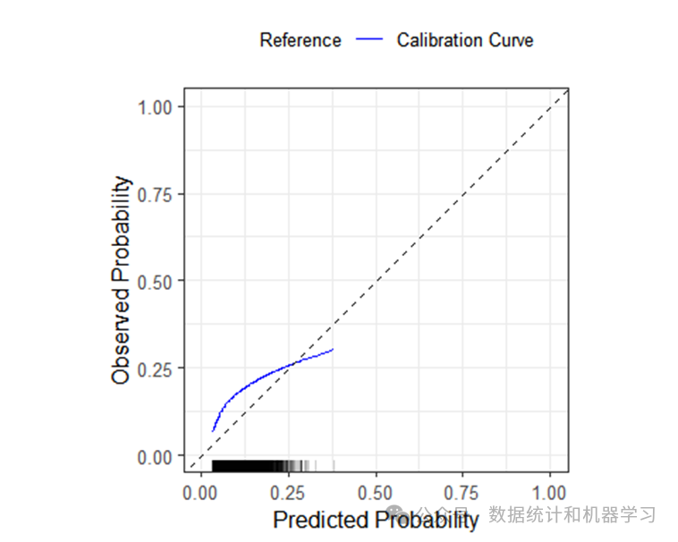

1.2 survival模型

survival模型，需要指定模型的累积风险以及回归系数。

​​​​​​​

coefs_table_2 <- data.frame("Age" = 0.007,                          "SexM" = 0.225,                          "Smoking_Status" = 0.685,                          "Diabetes" = 0.425,                          "Creatinine" = 0.587)
#构建模型Existing_TTE_Model <- pred_input_info(  model_type = "survival",  # 指定模型类型  model_info = coefs_table_2,  cum_hazard = SYNPM$TTE_mod1_baseline) # 累积风险

​​​​​​​

# 模型验证validation_results <- pred_validate(  x = Existing_TTE_Model,  new_data = SYNPM$ValidationData,  survival_time = "ETime",  event_indicator = "Status",  time_horizon = 5)

summary(validation_results)

# Calibration Measures # --------------------------------- #                         Estimate Std. Err Lower 95% Confidence Interval# Observed:Expected Ratio     1.22    0.011                          1.19# Calibration Slope           0.71    0.028                          0.66#                         Upper 95% Confidence Interval# Observed:Expected Ratio                          1.25# Calibration Slope                                0.77# #  Also examine the calibration plot, if produced. # # Discrimination Measures # --------------------------------- #           Estimate Std. Err Lower 95% Confidence Interval# Harrell C     0.58   0.0032                          0.57#           Upper 95% Confidence Interval# Harrell C                          0.59# #  Also examine the distribution plot of predicted risks. 

plot(validation_results)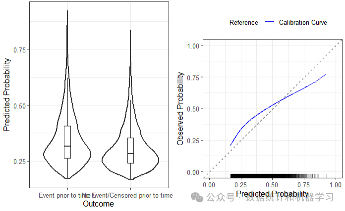

二、利用新数据集更新模型

2.1构建模型

​​​​​​​

coefs_table <- data.frame("Intercept" = -3.995,                           "Age" = 0.012,                          "SexM" = 0.267,                           "Smoking_Status" = 0.751,                          "Diabetes" = 0.523,                          "Creatinine" = 0.578)
Existing_Logistic_Model <- pred_input_info(  model_type = "logistic",  model_info = coefs_table)

2.2 更新模型（pred_updat（））

​​​​​​​

Updated_model <- pred_update(  Existing_Logistic_Model,  update_type = "recalibration",  new_data = SYNPM$ValidationData,  binary_outcome = "Y")

​​​​​​​

summary(Updated_model)# Original model was updated with type recalibration# The model updating results are as follows: # # Updated Model Coefficients # ================================= # # Model Functional Form # ================================= # Age + SexM + Smoking_Status + Diabetes + Creatinine

模型验证

​​​​​​​

pred_val <- pred_validate(  Updated_model,   new_data = SYNPM$ValidationData,   binary_outcome = "Y")summary(pred_val)

## Calibration Measures ## --------------------------------- ##                         Estimate Std. Err Lower 95% Confidence Interval## Observed:Expected Ratio        1   0.0188                        0.9638## Calibration Intercept          0   0.0204                       -0.0400## Calibration Slope              1   0.0713                        0.8603##                         Upper 95% Confidence Interval## Observed:Expected Ratio                        1.0375## Calibration Intercept                          0.0400## Calibration Slope                              1.1397## ##  Also examine the calibration plot, if produced. ## ## Discrimination Measures ## --------------------------------- ##     Estimate Std. Err Lower 95% Confidence Interval## AUC   0.5816   0.0057                        0.5703##     Upper 95% Confidence Interval## AUC                        0.5928## ## ## Overall Performance Measures ## --------------------------------- ## Cox-Snell R-squared: 0.0095## Nagelkerke R-squared: 0.0171## Brier Score: 0.1203## ##  Also examine the distribution plot of predicted risks.

绘制校准曲线

plot(pred_val)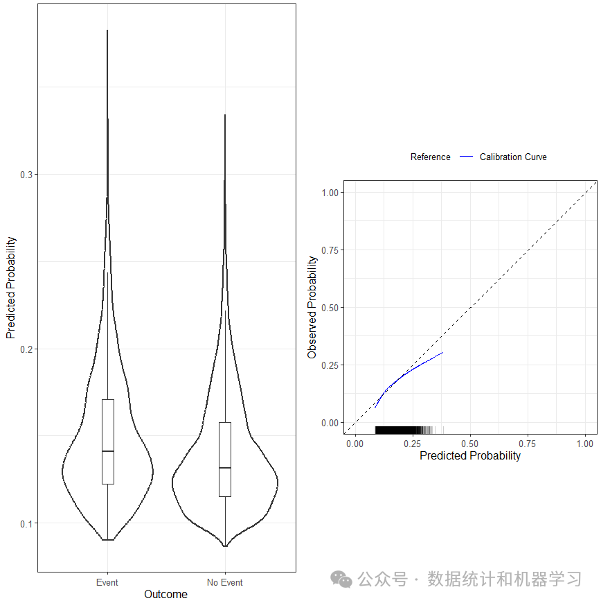

三、模型集成

当我们用模型集成时，元模型必须是同一类型的模型，比如logistic或survival模型，这与常用的模型集成有所不同。

构建集成模型

​​​​​​​

coefs_table <- data.frame(rbind(c("Intercept" = -3.995,                                  "Age" = 0.012,                                  "SexM" = 0.267,                                  "Smoking_Status" = 0.751,                                  "Diabetes" = 0.523,                                  "Creatinine" = 0.578),                                c("Intercept" = -2.282,                                  "Age" = NA,                                  "SexM" = 0.223,                                  "Smoking_Status" = 0.528,                                  "Diabetes" = 0.200,                                  "Creatinine" = 0.434),                                c("Intercept" = -3.013,                                  "Age" = NA,                                  "SexM" = NA,                                  "Smoking_Status" = 0.565,                                  "Diabetes" = -0.122,                                  "Creatinine" = 0.731)))multiple_mods <- pred_input_info(model_type = "logistic",                                 model_info = coefs_table)summary(multiple_mods)## Information about 3 existing model(s) of type 'logistic' ## ## Model Coefficients ## ================================= ## [[1]]##   Intercept   Age  SexM Smoking_Status Diabetes Creatinine## 1    -3.995 0.012 0.267          0.751    0.523      0.578## ## [[2]]##   Intercept  SexM Smoking_Status Diabetes Creatinine## 2    -2.282 0.223          0.528      0.2      0.434## ## [[3]]##   Intercept Smoking_Status Diabetes Creatinine## 3    -3.013          0.565   -0.122      0.731## ## ## Model Functional Form ## ================================= ## Model 1: Age + SexM + Smoking_Status + Diabetes + Creatinine## Model 2: SexM + Smoking_Status + Diabetes + Creatinine## Model 3: Smoking_Status + Diabetes + Creatinine

模型预测

SR <- pred_stacked_regression(x = multiple_mods,                              new_data = SYNPM$ValidationData,                              binary_outcome = "Y")summary(SR)## Existing models aggregated using stacked regression## The model stacked regression weights are as follows: ## (Intercept)         LP1         LP2         LP3 ##  0.02072515  0.48150208  0.12920227  0.16559034 ## ## Updated Model Coefficients ## ================================= ##   Intercept         Age      SexM Smoking_Status Diabetes Creatinine## 1 -2.696639 0.005778025 0.1573732      0.5233854 0.257464  0.4554285## ## Model Functional Form ## ================================= ## Age + SexM + Smoking_Status + Diabetes + Creatinine

模型验证​​​​​​​

pred_val_2 <- pred_validate(SR,               new_data = SYNPM$ValidationData,               binary_outcome = "Y")summary(pred_val_2)

​​​​​​​

# Calibration Measures # --------------------------------- #                         Estimate Std. Err# Observed:Expected Ratio        1   0.0188# Calibration Intercept          0   0.0204# Calibration Slope              1   0.0702#                         Lower 95% Confidence Interval# Observed:Expected Ratio                        0.9638# Calibration Intercept                         -0.0400# Calibration Slope                              0.8623#                         Upper 95% Confidence Interval# Observed:Expected Ratio                        1.0375# Calibration Intercept                          0.0400# Calibration Slope                              1.1377# #  Also examine the calibration plot, if produced. # # Discrimination Measures # --------------------------------- #     Estimate Std. Err Lower 95% Confidence Interval# AUC    0.583   0.0058                        0.5717#     Upper 95% Confidence Interval# AUC                        0.5943# # # Overall Performance Measures # --------------------------------- # Cox-Snell R-squared: 0.0098# Nagelkerke R-squared: 0.0175# Brier Score: 0.1203# #  Also examine the distribution plot of predicted risks.

绘制校准曲线

pred_val_2$flex_calibrationplot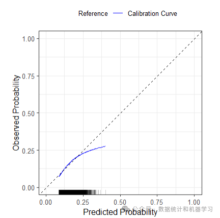

参考资料：https://glenmartin31.github.io/predRupdate