吴恩达Machine Learning课程对应Jupyter代码1‘（第一课 P1-41）Week1 持续更新

前面更新了吴恩达机器学习视频和对应笔记，接下来是对应的实验和代码测试，代码文件已附在笔记中，需要可下载，另外可结合教程笔记和知识点对照学习，以下第一课的笔记链接：

吴恩达Machine Learning课程学习笔记1（P1-41）-CSDN博客

欢迎交流学习，教程视频来自B站（P1-P41）吴恩达机器学习课程（第一课：Supervised Machine Learning Regression and Classification）：(超爽中英!) 2024公认最好的【吴恩达机器学习】教程！附课件代码 Machine Learning Specialization_哔哩哔哩_bilibili

---

目录

第一课 Supervised Machine Learning Regression and Classifications

Week1

Week1.1.overview of Machine Learning

Week1.2.Supervised vs Unsupervised Machine Learning

Week1.3.Practice Quiz Supervised vs unsupervised learning

Week1.4.Regression Model

Week1.5.Practice Quiz Regression Model

Week1.6.Train the model with gradient descent

Week1.7.Practice quiz Train the model with gradient descent

Week2

Week2.1.Multiple linear regression

Week2.2.Practice quiz Multiple linear regression

Week2.3.Gradient descent in practice

Week2.4.Practice quiz Gradient descent in practice

Week2.5.Week 2 practice lab Linear regression

Week3

Week3.1.Classification with logistic regression

Week3.2.Practice quiz Classification with logistic regression

Week3.3.Cost function for logistic regression

Week3.4.Practice quiz Cost function for logistic regression

Week3.5.Gradient descent for logistic regression

Week3.6.Practice quiz Gradient descent for logistic regression

Week3.7.The problem of overfitting

Week3.8.Practice quiz The problem of overfitting

Week3.9.Week 3 practice lab logistic regression

Week3.10.Acknowledgments

第二课 Advanced Learning Algorithms

Week1

Week1.1.Neural networks intuition

Week1.2.Practice quiz Neural networks intuition

Week1.3.Neural network model

Week1.4.Practice quiz Neural network model

Week1.5.TensorFlow implementation

Week1.6.Practice quiz TensorFlow implementation

Week1.7.Neural network implementation in Python

Week1.8.Neural network implementation in Python

Week1.9.Practice Lab Neural networks

Week2

Week2.1.Neural Network Training

Week2.2.Practice quiz Neural Network Training

Week2.3.Activation Functions

Week2.4.Practice quiz Activation Functions

Week2.5.Multiclass Classification

Week2.6 Practice quiz Multiclass Classification

Week2.7.Additional Neural Network Concepts

Week2.8.Practice quiz Additional Neural Network Concepts

Week2.9.Practice Lab Neural network training

Week3

Week3.1.Advice for applying machine learning

Week3.2.Practice quiz Advice for applying machine leaming

Week3.3.Bias and variance

Week3.4.Practice quiz Bias and variance

Week3.5.Machine learning development process

Week3.6.Practice quiz Machine learning development process

Week3.7.Skewed datasets (optional)

Week3.8.Practice Lab Advice for applying machine learning

Week4

Week4.1.Decision trees

Week4.2.Practice quiz Decision trees

Week4.3.Decision tree leamning

Week4.4.Practice quiz Decision tree leaming

Week4.5.Tree ensembles

Week4.6.Practice quiz Tree ensembles

Week4.7.Practice lab decision trees

---

第一课 Supervised Machine Learning Regression and Classifications

Week1

Week1.1.overview of Machine Learning

给自己补个进入jupyter的代码，方便copy：

cd "H:\1 宁的研究生资料\6 2024研二上 组会 小论文 大论文\4 中期前的准备工作\吴恩达机器学习教程相关资料\2024吴恩达资料\A最新版 吴恩达机器学习Deeplearning.ai"

 jupyter notebook 

cd /d H:\1 宁的研究生资料\6 2024研二上 组会 小论文 大论文\4 中期前的准备工作\吴恩达机器学习教程相关资料\2024吴恩达资料\A最新版 吴恩达机器学习Deeplearning.ai

Week1.2.Supervised vs Unsupervised Machine Learning

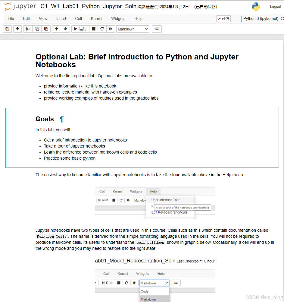
C1_W1_Lab01_Python_Jupyter_Soln(主要介绍插入Markdown/Code功能)

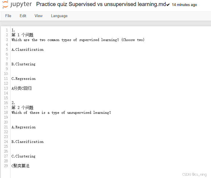
Week1.3.Practice Quiz Supervised vs unsupervised learning

Week1.4.Regression Model

C1_W1_Lab03_Model_Representation_Soln（单变量线性回归模型）

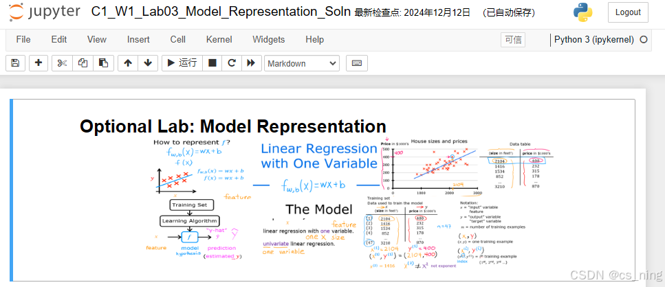
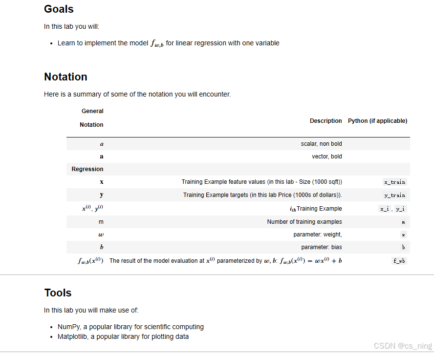
本次实验的目标是了解单变量线性回归fw,b，相关变量和代表的内容如上表，用到的工具是numpy和matplotlib。

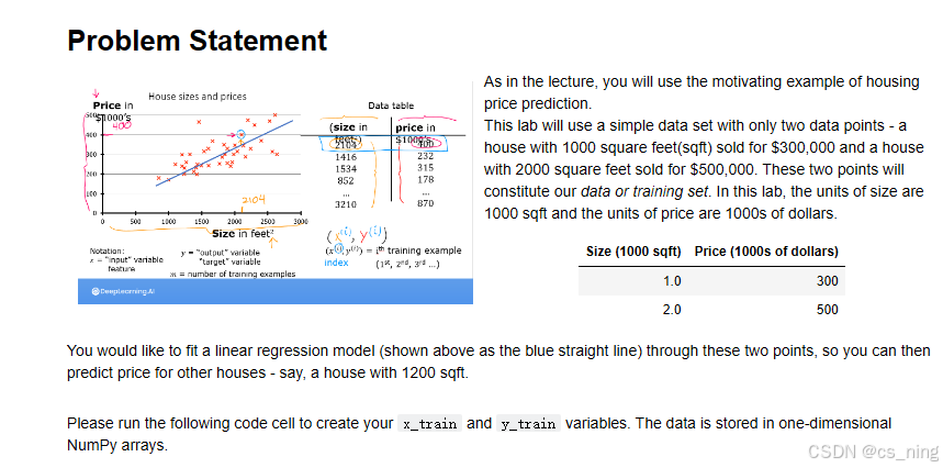
这次实验中使用一个简单的数据集，只有个数据点，一栋是1000平方英尺的房子售价30万美金、另一栋2000平方英尺售价50万美金，这两个数据构成数据集。

下面的代码是示意输入x、y，输出训练集数量和索引数据的方法。

import numpy as np
import matplotlib.pyplot as plt
plt.style.use('./deeplearning.mplstyle')

# x_train is the input variable (size in 1000 square feet)
# y_train is the target (price in 1000s of dollars)
x_train = np.array([1.0, 2.0])
y_train = np.array([300.0, 500.0])
print(f"x_train = {x_train}")
print(f"y_train = {y_train}")

# 这一步是输入x_train和y_train，数据存储在一维的数组中。
# x代表房子的尺寸，y代表房价。

# 这里列出输出训练集的数量的两种方式：

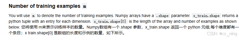
# 使用m来表示训练样本的数量。Numpy数组有一个.shape 参数，x_train.shape 返回一个 python 元组,每个维度都有一个条目；x train.shape[0] 是数组的长度和示例的数量，如下。

# m is the number of training examples
print(f"x_train.shape: {x_train.shape}")
m = x_train.shape[0]
print(f"Number of training examples is: {m}")


# 我们也可以用 len（）函数来计算，如下。

# m is the number of training examples
m = len(x_train)
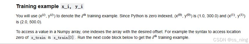
print(f"Number of training examples is: {m}")

# 这一步是尝试输出训练集的数据，我们用x(i) y(i)索引数据.
# 注意要访问Numpy数组中的值，数组是从[0]开始的，需要用所需的偏移量对数组进行索引。例如，访问x_train位置零的语法是x_train[0],运行下面的下一个代码块以获得培训示例。

i = 0 # Change this to 1 to see (x^1, y^1)

x_i = x_train[i]
y_i = y_train[i]
print(f"(x^({i}), y^({i})) = ({x_i}, {y_i})")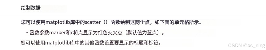

#这一步是将数据展示在图表中，代码运行结果如下

# Plot the data points
plt.scatter(x_train, y_train, marker='x', c='r')
# Set the title
plt.title("Housing Prices")
# Set the y-axis label
plt.ylabel('Price (in 1000s of dollars)')
# Set the x-axis label
plt.xlabel('Size (1000 sqft)')
plt.show()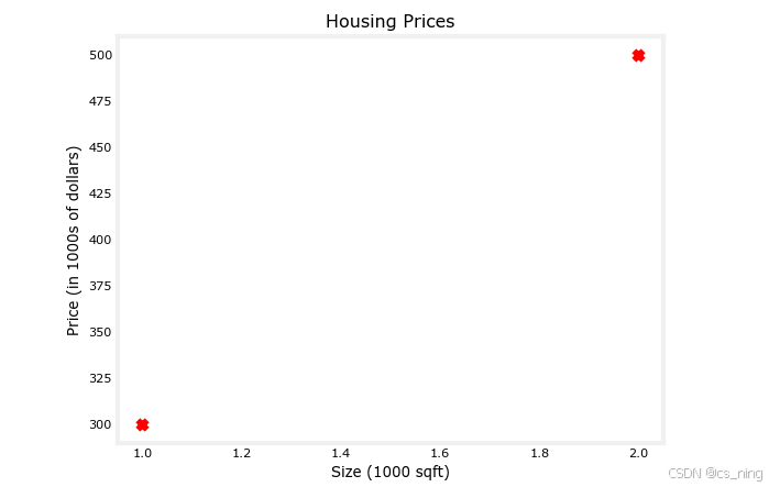

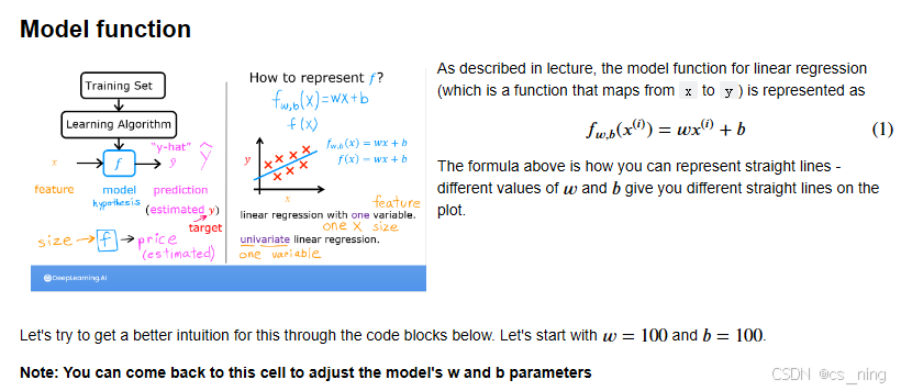
# 首先我们可以尝试赋予w,b初始值

w = 100
b = 100
print(f"w: {w}")
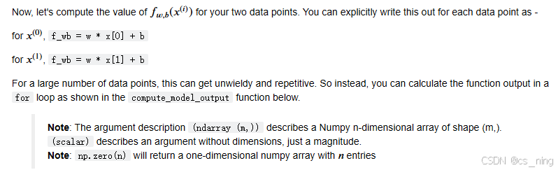
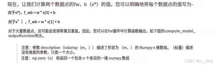
print(f"b: {b}")

# 接着计算两个数据点的fw,b值，可以借助for循环来输出。
# np.zero(n)将返回一个包含n个条目的一维numpy数组。
# 参数(ndarray(m，))描述了形状为(m.)的Numpy n维数组。(scalar)描述没有维度的参数，只是一个大小。


def compute_model_output(x, w, b):
    """
    Computes the prediction of a linear model
    Args:
      x (ndarray (m,)): Data, m examples 
      w,b (scalar)    : model parameters  
    Returns
      y (ndarray (m,)): target valu