图形可视化

library(ggplot2)
library(plotrix)
data("midwest", package = "ggplot2") #加载数据集
options(scipen=999)  # 关掉像 1e+48 这样的科学符号
# 颜色设置（灰色系列）
cbp1 <- c("#999999", "#E69F00", "#56B4E9", "#009E73",
          "#F0E442", "#0072B2", "#D55E00", "#CC79A7")

# 颜色设置（黑色系列）
cbp2 <- c("#000000", "#E69F00", "#56B4E9", "#009E73",
          "#F0E442", "#0072B2", "#D55E00", "#CC79A7")


ggplot <- function(...) ggplot2::ggplot(...) + 
  scale_color_manual(values = cbp1) +
  scale_fill_manual(values = cbp1) + # 注意: 使用连续色阶时需要重写
  theme_bw()
library(ggplot2)
library(ggdendro)
theme_set(theme_bw())

hc <- hclust(dist(USArrests), "ave")  # hierarchical clustering
# plot
ggdendrogram(hc, rotate = TRUE, size = 2)

# devtools::install_github("hrbrmstr/ggalt")
library(ggplot2)
library(ggalt)
library(ggfortify)
theme_set(theme_classic())

# Compute data with principal components ------------------
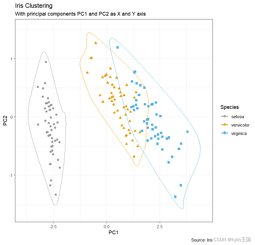
df <- iris[c(1, 2, 3, 4)]
pca_mod <- prcomp(df)  # compute principal components

# Data frame of principal components ----------------------
df_pc <- data.frame(pca_mod$x, Species=iris$Species)  # dataframe of principal components
df_pc_vir <- df_pc[df_pc$Species == "virginica", ]  # df for 'virginica'
df_pc_set <- df_pc[df_pc$Species == "setosa", ]  # df for 'setosa'
df_pc_ver <- df_pc[df_pc$Species == "versicolor", ]  # df for 'versicolor'

# Plot ----------------------------------------------------
ggplot(df_pc, aes(PC1, PC2, col=Species)) + 
  geom_point(aes(shape=Species), size=2) +   # draw points
  labs(title="Iris Clustering", 
       subtitle="With principal components PC1 and PC2 as X and Y axis",
       caption="Source: Iris") + 
  coord_cartesian(xlim = 1.2 * c(min(df_pc$PC1), max(df_pc$PC1)), 
                  ylim = 1.2 * c(min(df_pc$PC2), max(df_pc$PC2))) +   # change axis limits
  geom_encircle(data = df_pc_vir, aes(x=PC1, y=PC2)) +   # draw circles
  geom_encircle(data = df_pc_set, aes(x=PC1, y=PC2)) + 
  geom_encircle(data = df_pc_ver, aes(x=PC1, y=PC2))