


1、介绍
目的:分类还是回归?经典的二分类算法!
机器学习算法选择:先逻辑回归再用复杂的,能简单还是用简单的
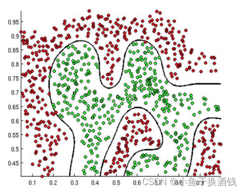
逻辑回归的决策边界:可以是非线性的
2、数学公式
2.1、Sigmoid 函数
公式:
自变量取值为任意实数,值域[0,1]

解释:将任意的输入映射到了[0,1]区间,我们在线性回归中可以得到一个预测值,再将该值映射到Sigmoid 函数中这样就完成了由值到概率的转换,也就是分类任务。
预测函数:
其中
2.2、分类任务
整合:
解释:对于二分类任务(0,1),整合后y取0只保留 ,y取1只保留
2.3、梯度下降求最优解
似然函数:
对数似然:
此时应用梯度上升求最大值,引入 转换为梯度下降任务
求导过程:
参数更新:
多分类的softmax:
3、代码实现
3.1、使用Scikit-learn库
直接使用Python的Scikit-learn库来实现逻辑回归算法
from sklearn.datasets import load_iris
from sklearn.linear_model import LogisticRegression

X, y = load_iris(return_X_y=True)

clf = LogisticRegression(random_state=0, solver='lbfgs', max_iter=10000,
                         multi_class='multinomial')
# 由于迭代更新次数太少,算法无法收敛,报错
clf.fit(X, y)

clf.predict(X[:2, :])

clf.predict_proba(X[:2, :])

result = clf.score(X, y)

print('Training Precision: {:5.4f}%'.format(result))
3.2、自己手写逻辑回归算法
①数据样例(csv)
param_1,param_2,validity
0.051267,0.69956,1
-0.092742,0.68494,1
0.18376,0.93348,0
0.22408,0.77997,0
②主函数类
import numpy as np
import pandas as pd
import matplotlib.pyplot as plt
import math

from logistic_regression import LogisticRegression
# 非线性分界的逻辑回归

"""数据格式
param_1,param_2,validity
0.051267,0.69956,1
-0.092742,0.68494,1
0.18376,0.93348,0
0.22408,0.77997,0
"""
data = pd.read_csv('../data/microchips-tests.csv')

# 类别标签
validities = [0, 1]

# 选择两个特征
x_axis = 'param_1'
y_axis = 'param_2'

# 散点图
for validity in validities:
    plt.scatter(
        data[x_axis][data['validity'] == validity],
        data[y_axis][data['validity'] == validity],
        label=validity
    )

plt.xlabel(x_axis)
plt.ylabel(y_axis)
plt.title('Microchips Tests')
# 图例
plt.legend()
plt.show()

# 行数
num_examples = data.shape[0]
x_train = data[[x_axis, y_axis]].values.reshape((num_examples, 2))
y_train = data['validity'].values.reshape((num_examples, 1))

# 训练参数
max_iterations = 100000
regularization_param = 0
polynomial_degree = 5
sinusoid_degree = 0
# 逻辑回归
logistic_regression = LogisticRegression(x_train, y_train, polynomial_degree)

# 训练
(thetas, costs) = logistic_regression.train(max_iterations)

columns = []
for theta_index in range(0, thetas.shape[1]):
    columns.append('Theta ' + str(theta_index));

# 训练结果
labels = logistic_regression.unique_labels

plt.plot(range(len(costs[0])), costs[0], label=labels[0])
plt.plot(range(len(costs[1])), costs[1], label=labels[1])

plt.xlabel('Gradient Steps')
plt.ylabel('Cost')
plt.legend()
plt.show()

# 预测
y_train_predictions = logistic_regression.predict(x_train)

# 准确率
precision = np.sum(y_train_predictions == y_train) / y_train.shape[0] * 100

print('Training Precision: {:5.4f}%'.format(precision))


num_examples = x_train.shape[0]
samples = 150
x_min = np.min(x_train[:, 0])
x_max = np.max(x_train[:, 0])

y_min = np.min(x_train[:, 1])
y_max = np.max(x_train[:, 1])

X = np.linspace(x_min, x_max, samples)
Y = np.linspace(y_min, y_max, samples)
Z = np.zeros((samples, samples))

# 结果展示
for x_index, x in enumerate(X):
    for y_index, y in enumerate(Y):
        data = np.array([[x, y]])
        Z[x_index][y_index] = logistic_regression.predict(data)[0][0]

positives = (y_train == 1).flatten()
negatives = (y_train == 0).flatten()

plt.scatter(x_train[negatives, 0], x_train[negatives, 1], label='0')
plt.scatter(x_train[positives, 0], x_train[positives, 1], label='1')
# 画等高线
plt.contour(X, Y, Z)

plt.xlabel('param_1')
plt.ylabel('param_2')
plt.title('Microchips Tests')
plt.legend()

plt.show()
③逻辑回归类logistic_regression.py
import numpy as np
from scipy.optimize import minimize
from utils.features import prepare_for_training
from utils.hypothesis import sigmoid


class LogisticRegression:
    def __init__(self, data, labels, polynomial_degree=0, normalize_data=False):
        """
        1.对数据进行预处理操作
        2.先得到所有的特征个数
        3.初始化参数矩阵
        """
        (data_processed,
         features_mean,
         features_deviation) = prepare_for_training(data, polynomial_degree, normalize_data=False)

        self.data = data_processed
        self.labels = labels
        # 对于一维数组(元组)或列表,unique函数去除其中重复的元素,并按元素由小到大的顺序返回一个新的无重复元素列表
        self.unique_labels = np.unique(labels)
        self.features_mean = features_mean
        self.features_deviation = features_deviation
        self.polynomial_degree = polynomial_degree
        self.normalize_data = normalize_data

        num_features = self.data.shape[1]
        num_unique_labels = np.unique(labels).shape[0]
        self.theta = np.zeros((num_unique_labels, num_features))

    def train(self, max_iterations=1000):
        cost_histories = []
        # 列数
        num_features = self.data.shape[1]
        # enumerate多用于在for循环中得到计数,利用它可以同时获得索引和值
        for label_index, unique_label in enumerate(self.unique_labels):
            current_initial_theta = np.copy(self.theta[label_index].reshape(num_features, 1))
            current_lables = (self.labels == unique_label).astype(float)
            (current_theta, cost_history) = LogisticRegression.gradient_descent(self.data, current_lables,
                                                                                current_initial_theta, max_iterations)
            self.theta[label_index] = current_theta.T
            cost_histories.append(cost_history)

        return self.theta, cost_histories

    @staticmethod
    def gradient_descent(data, labels, current_initial_theta, max_iterations):
        cost_history = []
        num_features = data.shape[1]
        # scipy.optimize.minimize(fun, x0, method=None, bounds=None, constraints=(), ...)
        # fun:目标函数,它的参数是待优化的参数向量。
        # x0:优化变量的初始向量。只能传数组
        # method:优化算法,包括BFGS、CG、L-BFGS-B等。
        # bounds:定义优化变量的边界。
        # constraints:定义优化变量的约束条件。
        result = minimize(
            # 要优化的目标:
            # lambda current_theta:LogisticRegression.cost_function(data,labels,current_initial_theta.reshape(num_features,1)),
            lambda current_theta: LogisticRegression.cost_function(data, labels,
                                                                   current_theta.reshape(num_features, 1)),
            # 初始化的权重参数
            current_initial_theta.flatten(),
            # 选择优化策略
            method='CG',
            # 梯度下降迭代计算公式
            # jac = lambda current_theta:LogisticRegression.gradient_step(data,labels,current_initial_theta.reshape(num_features,1)),
            jac=lambda current_theta: LogisticRegression.gradient_step(data, labels,
                                                                       current_theta.reshape(num_features, 1)),
            # 记录结果
            callback=lambda current_theta: cost_history.append(
                LogisticRegression.cost_function(data, labels, current_theta.reshape((num_features, 1)))),
            # 迭代次数
            options={'maxiter': max_iterations}
        )
        if not result.success:
            raise ArithmeticError('Can not minimize cost function' + result.message)
        optimized_theta = result.x.reshape(num_features, 1)
        return optimized_theta, cost_history

    @staticmethod
    def cost_function(data, labels, theat):
        num_examples = data.shape[0]
        predictions = LogisticRegression.hypothesis(data, theat)
        y_is_set_cost = np.dot(labels[labels == 1].T, np.log(predictions[labels == 1]))
        y_is_not_set_cost = np.dot(1 - labels[labels == 0].T, np.log(1 - predictions[labels == 0]))
        cost = (-1 / num_examples) * (y_is_set_cost + y_is_not_set_cost)
        return cost

    @staticmethod
    def hypothesis(data, theat):

        predictions = sigmoid(np.dot(data, theat))

        return predictions

    @staticmethod
    def gradient_step(data, labels, theta):
        num_examples = labels.shape[0]
        predictions = LogisticRegression.hypothesis(data, theta)
        label_diff = predictions - labels
        gradients = (1 / num_examples) * np.dot(data.T, label_diff)

        # flatten()是对多维数据的降维函数。
        return gradients.T.flatten()

    def predict(self, data):
        num_examples = data.shape[0]
        data_processed = prepare_for_training(data, self.polynomial_degree,  self.normalize_data)[0]
        # 这边得到的是[(结果是0的概率,结果是1的概率)],所以才在下面取概率较大的值为预测结果
        prob = LogisticRegression.hypothesis(data_processed, self.theta.T)
        # 较大的数在第几列
        max_prob_index = np.argmax(prob, axis=1)
        class_prediction = np.empty(max_prob_index.shape, dtype=object)
        for index, label in enumerate(self.unique_labels):
            class_prediction[max_prob_index == index] = label
        return class_prediction.reshape((num_examples, 1))
④初始化数据normalize.py
这里并没有用到,略。
⑤数据处理prepare_for_training.py
"""Prepares the dataset for training"""

import numpy as np
# . 表示导入当前文件夹下的包
from .normalize import normalize
from .generate_sinusoids import generate_sinusoids
from .generate_polynomials import generate_polynomials


def prepare_for_training(data, polynomial_degree=0, normalize_data=True):

    # 计算样本总数
    num_examples = data.shape[0]

    data_processed = np.copy(data)

    # 预处理
    features_mean = 0
    features_deviation = 0
    data_normalized = data_processed
    if normalize_data:
        (
            data_normalized,
            features_mean,
            features_deviation
        ) = normalize(data_processed)

        data_processed = data_normalized


    # 特征变换polynomial
    if polynomial_degree > 0:
        polynomials = generate_polynomials(data_normalized, polynomial_degree, normalize_data)
        data_processed = np.concatenate((data_processed, polynomials), axis=1)

    # 加一列1
    # np.hstack:水平(按列顺序)把数组给堆叠起来,vstack()函数正好和它相反
    data_processed = np.hstack((np.ones((num_examples, 1)), data_processed))

    return data_processed, features_mean, features_deviation
⑥特征变换generate_polynomials.py
"""Add polynomial features to the features set"""

import numpy as np
from .normalize import normalize


def generate_polynomials(dataset, polynomial_degree, normalize_data=False):
    """变换方法:
    x1, x2, x1^2, x2^2, x1*x2, x1*x2^2, etc.
    """

    # 按行(竖向)将一个数组拆分为多个。返回的是一个数组,其中包含多个数组
    features_split = np.array_split(dataset, 2, axis=1)
    dataset_1 = features_split[0]
    dataset_2 = features_split[1]

    (num_examples_1, num_features_1) = dataset_1.shape
    (num_examples_2, num_features_2) = dataset_2.shape

    if num_examples_1 != num_examples_2:
        raise ValueError('Can not generate polynomials for two sets with different number of rows')

    if num_features_1 == 0 and num_features_2 == 0:
        raise ValueError('Can not generate polynomials for two sets with no columns')

    if num_features_1 == 0:
        dataset_1 = dataset_2
    elif num_features_2 == 0:
        dataset_2 = dataset_1

    num_features = num_features_1 if num_features_1 < num_examples_2 else num_features_2
    # 获取二维数组的所有行和num_features数量的列
    dataset_1 = dataset_1[:, :num_features]
    dataset_2 = dataset_2[:, :num_features]

    # 返回一个(num_examples_1, 0)维度的数值,里面的数据并不一定都为空
    polynomials = np.empty((num_examples_1, 0))

    for i in range(1, polynomial_degree + 1):
        for j in range(i + 1):
            polynomial_feature = (dataset_1 ** (i - j)) * (dataset_2 ** j)
            # 语法:concatenate((a1, a2, …), axis=0)
            # 说明:(a1, a2, …)为待拼接的数据,可以是一维,也可以是多维。
            # axis决定着怎么将数据拼接:axis=0是将数据按列拼接(即竖着拼接);
            # axis=1是将数据按行拼接(即横着拼接);
            # axis=None则是先将数据拉成一维向量,再拼接。
            polynomials = np.concatenate((polynomials, polynomial_feature), axis=1)

    if normalize_data:
        polynomials = normalize(polynomials)[0]

    return polynomials
⑥运行结果
需要分类的数据
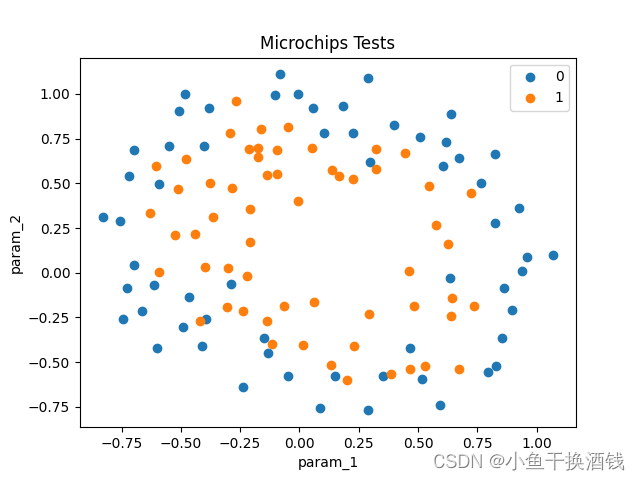
训练过程中的损失值

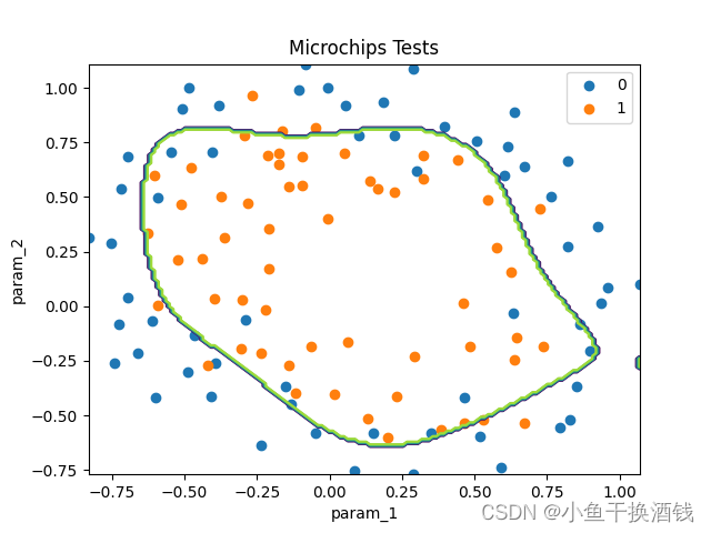
分类结果
4、总结
常用于二分类。
最后,觉得有帮助或者有点收获的话,帮忙点个赞吧!


 1226
1226


 被折叠的 条评论
为什么被折叠?
被折叠的 条评论
为什么被折叠?
 到【灌水乐园】发言


