R语言：方差分析，单因素方差分析，单个协变量的单因素方差分析，双因素方差分析，多元方差分析

最新推荐文章于 2024-04-24 11:17:03 发布

muyi沐一

最新推荐文章于 2024-04-24 11:17:03 发布

阅读量1.5k

点赞数 1

分类专栏： R语言文章标签： r语言学习

本文链接：https://blog.csdn.net/weixin_48293076/article/details/127181077

版权

R语言专栏收录该内容

10 篇文章 2 订阅

订阅专栏

方差分析包括：

在这里插入图片描述

各种方差分析表达公式设计

在这里插入图片描述
！！！注意，这里很强调顺序，这里的A、B是因素（也可以说是自变量），y是因变量，但是x 不是自变量，而是协变量（不是主要因素但是会对结果有一定的影响）

！！！有协变量的情况，协变量因素写在主变量前

单因素方差分析

> library(multcomp)
> cholesterol
      trt response
1   1time   3.8612
2   1time  10.3868
3   1time   5.9059
4   1time   3.0609
5   1time   7.7204
6   1time   2.7139
7   1time   4.9243
8   1time   2.3039
9   1time   7.5301
10  1time   9.4123
11 2times  10.3993
12 2times   8.6027
13 2times  13.6320
14 2times   3.5054
15 2times   7.7703
16 2times   8.6266
17 2times   9.2274
18 2times   6.3159
19 2times  15.8258
20 2times   8.3443
21 4times  13.9621
22 4times  13.9606
23 4times  13.9176
24 4times   8.0534
25 4times  11.0432
26 4times  12.3692
27 4times  10.3921
28 4times   9.0286
29 4times  12.8416
30 4times  18.1794
31  drugD  16.9819
32  drugD  15.4576
33  drugD  19.9793
34  drugD  14.7389
35  drugD  13.5850
36  drugD  10.8648
37  drugD  17.5897
38  drugD   8.8194
39  drugD  17.9635
40  drugD  17.6316
41  drugE  21.5119
42  drugE  27.2445
43  drugE  20.5199
44  drugE  15.7707
45  drugE  22.8850
46  drugE  23.9527
47  drugE  21.5925
48  drugE  18.3058
49  drugE  20.3851
50  drugE  17.3071
> names(cholesterol)
[1] "trt"      "response"
> attach(cholesterol)  #绑定数据框
> table(trt)
trt
 1time 2times 4times  drugD  drugE 
    10     10     10     10     10 
> aggregate(response,by=list(trt),FUN=mean)#先利用每组均值看一下药物作用的结果
  Group.1        x
1   1time  5.78197
2  2times  9.22497
3  4times 12.37478
4   drugD 15.36117
5   drugE 20.94752
#由结果可以看出drugE药物结果作用的效果最好

#我们用方差分析看一下，每组间作用效果差异性是否显著
> fit <- aov(response~trt,cholesterol)
> fit
Call:
   aov(formula = response ~ trt, data = cholesterol)

Terms:
                      trt Residuals
Sum of Squares  1351.3690  468.7504
Deg. of Freedom         4        45

Residual standard error: 3.227488
Estimated effects may be unbalanced

> summarry(fit)
Error in summarry(fit) : could not find function "summarry"
> summary(fit)   #主要看F值和P值
            Df Sum Sq Mean Sq F value   Pr(>F)    
trt          4 1351.4   337.8   32.43 9.82e-13 ***
Residuals   45  468.8    10.4                     
---
Signif. codes:  0 ‘***’ 0.001 ‘**’ 0.01 ‘*’ 0.05 ‘.’ 0.1 ‘ ’ 1
> par(mfrow=c(2,2))
> plot(fit)

F值越大组间差异越显著，P值越小F值越可靠

在这里插入图片描述
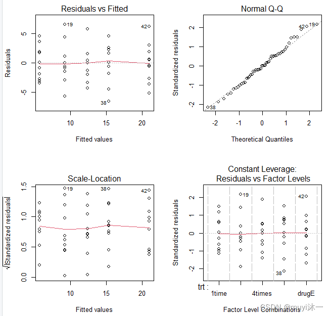
分析一下图，plot()函数作用后会出现4幅图

1、Residuals vs Fitted
检验残差与估计值是否有关（最佳状态散乱分布无关）。
Resiuals即为残差的意思（估计值与真实值之差）。这就是残差与真实值之间的关系画图。在理想线性模型中有五大假设。其中之一便是残差应该是一个正态分布，与估计值无关。如果残差还和估计值有关，那就说明模型仍然有值得去改进的地方，当然，这样的模型准确程度也就大打折扣。
所以点与线是散乱排布的，没有融合趋势的，这样的效果是好的

2、Normal QQ
Normal QQ-plot用来检测其残差是否是正态分布的。
如果呈现正态性，图形应该是一条近似与直线的线（有上升趋势）。

3、Scale-Location
这个图是用来检查等方差假设的，最佳状态红色的线应该趋近于水平。
在一开始我们的五大假设第二条便是，我们假设预测的模型里方差是一个定值。如果方差不是一个定值那么这个模型的可靠性也是大打折扣的。

4、Constant Leverage
一般当各点的标准差集种在0处且分布较为均匀时，则说明拟合结果较好。

另外补充一下，如果是用plot()函数分析lm()回归结果时，前三幅图与上面一样，不一样的是第四幅图，回归分析时第四幅图是

Residuals vs Leverage
Leverage就是杠杆的意思。这种图的意义在于检查数据分析项目中是否有特别极端的点。
在这里我们引入了一个非常重要的指标：Cook距离。我们在线性模型里用Cook距离分析一个点是否非常“influential。”一般来说距离大于0.5的点就需要引起注意了。在这里我们借用了物理学电磁场理论中的等电势理念。那个1，和0.5分别就是Cook距离为1和0.5的等高线。

lm()函数也可以用来做方差的分析

单个协变量的单因素方差分析

协变量不是探讨的主要因素但是有对结果因变量有一定的影响

#这里用litter数据集，
#dose是药物剂量主要研究因素，
#weight是出生体重因变量，
#gettime是怀孕时间是协变量
> names(litter)
[1] "dose"     "weight"   "gesttime" "number"  
> table(litter$dose)

  0   5  50 500 
 20  19  18  17 
> #再分组统计一下平均数
> attach(litter)
> aggregate(weight,by=list(dose),mean)
  Group.1        x
1       0 32.30850
2       5 29.30842
3      50 29.86611
4     500 29.64647
> #查看一下组间是否是显著的差别
> #总时间gesttime有差别，会影响到结果，属于协变量
> fit<- aov(weight~gesttime+dose,data = litter)
> fit
Call:
   aov(formula = weight ~ gesttime + dose, data = litter)

Terms:
                 gesttime      dose Residuals
Sum of Squares   134.3039  137.1229 1151.2718
Deg. of Freedom         1         3        69

Residual standard error: 4.08474
Estimated effects may be unbalanced
> summary(fit)
            Df Sum Sq Mean Sq F value  Pr(>F)   
gesttime     1  134.3  134.30   8.049 0.00597 **
dose         3  137.1   45.71   2.739 0.04988 * 
Residuals   69 1151.3   16.69                   
---
Signif. codes:  0 ‘***’ 0.001 ‘**’ 0.01 ‘*’ 0.05 ‘.’ 0.1 ‘ ’ 1
#结果表明怀孕时间与出生体重相关，控制怀孕时间药物剂量与出生体重是有影响的（一颗星）

双因素方差分析

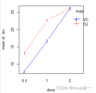
使用数据集ToothGrowth，这个数据集是利用60只小鼠，分别采用两种测试方法（橙汁，VC），每种方法中抗血栓含量dose有三种水平0.5，1，2，牙齿长度len是因变量，supp是选用方法分类
这里的双因素一个是食用方法（橙汁，VC），一个是剂量（0.5，1，2）

因变量必须是数值型numeric，主因素为因子类型factor

> names(ToothGrowth)
[1] "len"  "supp" "dose"
> attach(ToothGrowth)
> #统计一下频率
> xtabs(~supp+dose)
    dose
supp 0.5  1  2
  OJ  10 10 10
  VC  10 10 10
> #看一下平均值可否可以看出差别
> aggregate(len,by=list(supp,dose),mean)
  Group.1 Group.2     x
1      OJ     0.5 13.23
2      VC     0.5  7.98
3      OJ     1.0 22.70
4      VC     1.0 16.77
5      OJ     2.0 26.06
6      VC     2.0 26.14
> #可以看出剂量越小两用使用方法的差别越大
> #aov的对象为因子，这里我们应该先转化数据类型
> class(ToothGrowth$dose)
[1] "numeric"
> class(ToothGrowth$len) #因变量是数值型不需要变化
[1] "numeric"
> ToothGrowth$dose <- factor(ToothGrowth$dose)
> class(ToothGrowth$dose)
[1] "factor"
> fit <- aov(len~supp*dose,data=ToothGrowth)
> fit
Call:
   aov(formula = len ~ supp * dose, data = ToothGrowth)

Terms:
                    supp     dose supp:dose Residuals
Sum of Squares   205.350 2426.434   108.319   712.106
Deg. of Freedom        1        2         2        54

Residual standard error: 3.631411
Estimated effects may be unbalanced
> summary(fit)
            Df Sum Sq Mean Sq F value   Pr(>F)    
supp         1  205.4   205.4  15.572 0.000231 ***
dose         2 2426.4  1213.2  92.000  < 2e-16 ***
supp:dose    2  108.3    54.2   4.107 0.021860 *  
Residuals   54  712.1    13.2                     
---
Signif. codes:  0 ‘***’ 0.001 ‘**’ 0.01 ‘*’ 0.05 ‘.’ 0.1 ‘ ’ 1

#supp、dose后面都是三颗星，说明结果显著，都有影响
#可视化展示可以用HH包中的interaction.plot()绘图
> install.packages("HH")
> interaction.plot(dose,supp,len,type = "b",
+                  col=c("red","blue",pch=c(16,18),
+                  main="Interaction between Dose and Supplement Type"))

在这里插入图片描述

多元方差分析

研究的是美国谷物里的卡路里、脂肪和糖类含量是否因为储物架的不同而有影响
shelf代表货架，1低货架；2中层货架；3顶层货架
卡路里、脂肪和糖类含量是因变量，货架水平是自变量

多个因变量y时，无论是进行计算均值还是计算多元方差分析都要将众多y合并用 cbind(y1,y2……)函数

> library(MASS)
> names(UScereal)
 [1] "mfr"       "calories"  "protein"   "fat"      
 [5] "sodium"    "fibre"     "carbo"     "sugars"   
 [9] "shelf"     "potassium" "vitamins" 
> attach(UScereal)
> #需要将shelf列转化为因子
> class(UScereal$shelf)
[1] "integer"
> UScereal$shelf <- factor(UScereal$shelf)
> class(UScereal$shelf)
[1] "factor"
> #分组统计一下平均值
> aggregate(calories,fat,sugars,by=list(shelf),FUN=mean)
Error in mean.default(X[[i]], ...) : 'trim'必需是长度必需为一的数值
In addition: Warning message:
In if (na.rm) x <- x[!is.na(x)] :
  the condition has length > 1 and only the first element will be used
> #这里报错是因为aggregate只能输入一个变量
> aggregate(cbind(calories,fat,sugars),by=list(shelf),FUN=mean)
  Group.1 calories       fat    sugars
1       1 119.4774 0.6621338  6.295493
2       2 129.8162 1.3413488 12.507670
3       3 180.1466 1.9449071 10.856821
> #有多个y因变量，需要合并着表示
> fit <- manova(cbind(calories,fat,sugars)~shelf)
> fit
Call:
   manova(cbind(calories, fat, sugars) ~ shelf)

Terms:
                   shelf Residuals
calories         45313.4  203982.1
fat                18.42    155.24
sugars            183.34   1995.87
Deg. of Freedom        1        63

Residual standard errors: 56.90177 1.569734 5.628535
Estimated effects may be unbalanced
> summary(fit)
          Df  Pillai approx F num Df den Df  Pr(>F)   
shelf      1 0.19594    4.955      3     61 0.00383 **
Residuals 63                                          
---
Signif. codes:  0 ‘***’ 0.001 ‘**’ 0.01 ‘*’ 0.05 ‘.’ 0.1 ‘ ’ 1
> #可使用summary.aov()函数分别查看因素对每个因变量的影响
> summary.aov(fit)
 Response calories :
            Df Sum Sq Mean Sq F value    Pr(>F)    
shelf        1  45313   45313  13.995 0.0003983 ***
Residuals   63 203982    3238                      
---
Signif. codes:  0 ‘***’ 0.001 ‘**’ 0.01 ‘*’ 0.05 ‘.’ 0.1 ‘ ’ 1

 Response fat :
            Df  Sum Sq Mean Sq F value   Pr(>F)   
shelf        1  18.421 18.4214   7.476 0.008108 **
Residuals   63 155.236  2.4641                    
---
Signif. codes:  0 ‘***’ 0.001 ‘**’ 0.01 ‘*’ 0.05 ‘.’ 0.1 ‘ ’ 1

 Response sugars :
            Df  Sum Sq Mean Sq F value  Pr(>F)  
shelf        1  183.34  183.34   5.787 0.01909 *
Residuals   63 1995.87   31.68                  
---
Signif. codes:  0 ‘***’ 0.001 ‘**’ 0.01 ‘*’ 0.05 ‘.’ 0.1 ‘ ’ 1