


一、 使用PyTorch构建LeNet模型
# 构建网络层 --> LeNet
import torch.nn as nn
class LeNet(nn.Module):
    def __init__(self):
        super(LeNet,self).__init__()
        self.conv1 = nn.Conv2d(1, 6, 5) # 1:灰度图片的通道, 6: 输出通道, 5:kernel
        self.conv2 = nn.Conv2d(6, 16, 3) # 6:输入通道, 16:输出通道, 3:kernel
        self.fc1 = nn.Linear(16*5*5, 120) # 16*5*5:输入通道, 120:输出通道
        self.fc2 = nn.Linear(120, 84) # 120:输入通道, 84:输出通道
        self.fc3 = nn.Linear(84, 10) # 输入84,输出10


    def forward(self, x):
        input_size = x.size(0) # batch_size
        x = self.conv1(x) # 输入:batch*1*28*28, 输出:batch*6*24*24 (28 -5 +1 = 24)
        x = F.leaky_relu(x,negative_slope=0.1) # 激活函数
        x = F.max_pool2d(x, 2, 2) # 输入:batch*6*24*24, 输出:batch*6*12*12

        x = self.conv2(x) # 输入:batch*6*12*12, 输出batch*16*10*10 (12 -3 +1 = 10)
        x = F.leaky_relu(x, negative_slope=0.1) # 激活函数
        x = F.max_pool2d(x, 2, 2) # 输入batch*16*10*10, 输出batch*16*5*5

        x = x.view(input_size, -1) # 拉平(一列)
#         print("data shape",len(x),x.size(), x)

        x = self.fc1(x) # 输入:batch*16*6*5, 输出:batch*120
        x = F.leaky_relu(x,negative_slope=0.1) #保持shape不变

        x = self.fc2(x) # 输入:batch*120, 输出:batch*84
        x = F.relu(x) # 保持不变

        output = self.fc3(x) #输入:batch*84, 输出:batch*10

        #output = F.log_softmax(x, dim=1) # 计算分类后,每个数字的概率值

        return output
二、自定义方法(1、读取数据集2、划分批次3、显示图片4、数据预处理)并验证
1、读取数据集
# 导入模块
import numpy as np
import gzip
import os
import matplotlib.pyplot as plt

# 1、定义读取压缩文件数据的函数
def decompression_function(data_folder, data_name, label_name):
    with gzip.open(os.path.join(data_folder,label_name), 'rb') as lbpath: # rb表示的是读取二进制数据
        y_train = np.frombuffer(lbpath.read(), np.uint8, offset=8)

    with gzip.open(os.path.join(data_folder,data_name), 'rb') as imgpath:
        x_train = np.frombuffer(
            imgpath.read(), np.uint8, offset=16).reshape(len(y_train), 28, 28)
    return x_train, y_train


file_path = './data/MNIST/raw'

train_image_gz_path = "train-images-idx3-ubyte.gz"
train_label_gz_path = "train-labels-idx1-ubyte.gz"
train_image, train_label = decompression_function(file_path, train_image_gz_path, train_label_gz_path)
print("训练集:\n", "图片:", len(train_image), "标签:", len(train_label))

val_image_gz_path = "t10k-images-idx3-ubyte.gz"
val_label_gz_path = "t10k-labels-idx1-ubyte.gz"
val_image, val_label = decompression_function(file_path, val_image_gz_path, val_label_gz_path)
print("验证集:\n", "图片:", len(val_image), "标签:", len(val_label))

2、定义划分批次的函数:
# 2、定义划分批次的函数
def batch_split(data, label, batch_size):
    samples = data.shape[0]
    #print(data.shape,samples)
    data_list, label_list = [], []
    times = samples // batch_size if samples % batch_size == 0 else samples // batch_size + 1
    # times = samples //batch
    for i in range(times):
        start = i * batch_size
        end = start + batch_size
        batch_data = data[start:end,: , :]
        batch_label = label[start:end]
        data_list.append(batch_data)
        label_list.append(batch_label)
        #print(i,":",start,end)
        #print(data[start:end,:]
    return data_list, label_list


#划分每一批次,批次大小为 64
# 训练集
train_data,train_labels = batch_split(train_image, train_label, 64)
# 验证集
val_data,val_labels = batch_split(val_image, val_label, 64)
# 打印
print("data:\n",train_data,"\n","label:\n",train_labels)
print("data:\n",val_data,"\n","label:\n",val_labels)
3、定义显示批次图片函数:
#3、显示第一批的每张图片
def img_show(x,y,suptitle):
first_batch_image = x[0]
first_batch_label = y[0]
for i in range(len(first_batch_image)):
img = first_batch_image[i]
plt.subplot(8,8,i+1)
plt.imshow(img)
plt.title(str(first_batch_label[i]))
plt.axis("off")
plt.suptitle(suptitle, y=1.7,fontsize = 30)
plt.subplots_adjust(top=1.5)
plt.show()
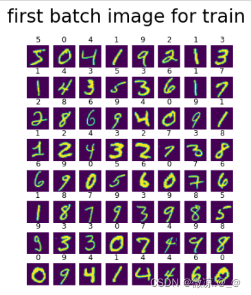
# 显示第一批训练集的每张图片
suptitle = "first batch image for train"
img_show(train_data,train_labels,suptitle)
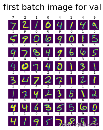
#显示第一批次验证集的每张图片
suptitle = "first batch image for val"
img_show(val_data,val_labels,suptitle)
显示的图片(第一批次):
4、数据预处理: --> 1、批量标准化处理 2、转为tensor 格式 3、shape 改为 [x,1,28,28]
# 4、数据预处理 --> 1、批量标准化处理 2、转为tensor 格式 3、shape 改为 [x,1,28,28]
import torch
def data_process(batch_data):
    result_batch = 0.0
    if len(batch_data.shape) > 1:    # 判断输入是 data 还是 label
        # data
        batch_all_data = []
        for i in batch_data:
            for k in i:
                for j in k:
                    batch_all_data.append(j)

        batch_mean = np.array(batch_all_data).mean()
        batch_std = np.array(batch_all_data).std()
        # 批量标准化处理
        batch_Normalize = (batch_data-batch_mean) / batch_std
        # 转为tensor格式
        batch_to_tensor = torch.from_numpy(batch_Normalize).type(torch.float32)
        # shape 改为 [x,1,28,28]
        result_batch = torch.unsqueeze(batch_to_tensor,dim=1)


    else:
        # label
        result_batch = torch.from_numpy(batch_data)


    return result_batch
三、自定义对比损失函数–>CrossEntropy()
# 定义损失函数-->CrossEntropyLoss()
import torch.nn.functional as F
def crossentropyloss(predict, y):
    # log_softmax
    softmax_x = F.softmax(predict, dim=1)
    log_softmax_x = torch.log(softmax_x)
    # nllloss
    batch_loss = F.nll_loss(log_softmax_x,y,reduction="mean")

    return batch_loss
四、TSNE可视化
# 2d
import numpy as np
import matplotlib.pyplot as plt
from mpl_toolkits.mplot3d import Axes3D
from sklearn.manifold import TSNE


X = np.reshape(train_image,(60000,784))[:1000,:]
y = train_label[:1000]

tsne = TSNE(n_components=3, random_state=0)

X_2d = tsne.fit_transform(X)

target_ids = range(len(X))


plt.figure(figsize=(6, 5))

colors = 'r', 'g', 'b', 'c', 'm', 'y', 'k', 'w', 'orange', 'purple'

for i, c, label in zip(target_ids, colors, np.unique(y)):

    plt.scatter(X_2d[y == i, 0], X_2d[y == i, 1], c=c, label=label)

plt.title("t-SNE 2D")
plt.legend()
plt.show()
可视化2d图片:

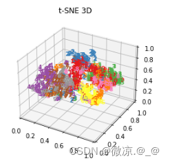
# 3d
X_3d = tsne.fit_transform(X)
def plot_embedding_3d(X, title=None):
    #坐标缩放到[0,1]区间
    x_min, x_max = np.min(X,axis=0), np.max(X,axis=0)
    X = (X - x_min) / (x_max - x_min)
    #降维后的坐标为(X[i, 0], X[i, 1],X[i,2]),在该位置画出对应的digits
    fig = plt.figure()
    ax = fig.add_subplot(1, 1, 1, projection='3d')
    for i in range(X.shape[0]):
        ax.text(X[i, 0], X[i, 1], X[i,2],str(y[i]),
                 color=plt.cm.Set1(y[i] / 10.),
                 fontdict={'weight': 'bold', 'size': 9})
    if title is not None:
        plt.title(title)

plot_embedding_3d(X_3d,"t-SNE 3D " )
可视化3d图片:
五、定义超参数,训练模型
#定义超参数
import torch.optim as optim
epochs = 15 #训练数据集的轮次
#batch_size = 64 #每批处理的数据
device = torch.device("cuda" if torch.cuda.is_available() else "cpu")
print(device)
model = LeNet().to(device)
optimizer = optim.Adam(model.parameters())
# 训练模型
def train_val(model,x_train,y_train,x_val,y_val,epochs):
val_accuracy = [] #储存每一轮验证集准确率
train_batch_loss = [] #储存每一批次训练集loss
val_batch_loss = [] #储存每一批次验证集loss
for epoch in range(epochs):
model.train()
for batch_t in range(len(x_train)):
# data_process() 数据预处理 --> 1、批量标准化处理 2、转为tensor 格式 3、shape 改为 [64,1,28,28]
data_t = data_process(x_train[batch_t])
traget_t = data_process(y_train[batch_t])
#部署到DEVICE上去
data_t, traget_t = data_t.to(device), traget_t.to(device)
# print("数据尺寸:",data_t.shape)
# print("标签尺寸:",traget_t.shape)
# # 梯度初始化为0
optimizer.zero_grad()
# # 训练后的结果
output = model(data_t)
# print("输出尺寸",output.shape)
# # 计算损失
loss = F.cross_entropy(output, traget_t)
myloss = crossentropyloss(output, traget_t) #自定义损失函数
train_batch_loss.append(myloss.item())
# print("损失:",loss)
# #反向传播
loss.backward()
# # 参数优化
optimizer.step()
# print(batch_t,batch_t % 3000 == 0)
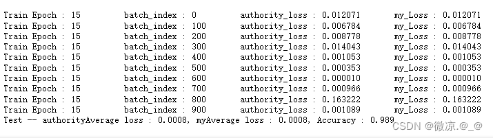
if batch_t % 100 == 0:
print("Train Epoch : {} \t batch_index : {} \t authority_loss : {:.6f} \t my_Loss : {:.6f}".format(epoch+1,
batch_t,
loss.item(),
myloss.item()))
#模型验证
model.eval()
#正确率
correct = 0.0
#测试损失
test_loss = 0.0
mytest_loss = 0.0
len_batch = 0
with torch.no_grad(): # 不会计算梯度,也不会进行反向传播
for batch_v in range(len(x_val)):
len_batch += len(x_val[batch_v]) #计算验证集数据总条数
data_v = data_process(x_val[batch_v])
target_v = data_process(y_val[batch_v])
# 部署到device上
data_v, target_v = data_v.to(device), target_v.to(device)
# 测试数据
output = model(data_v)
# 计算测试损失
val_loss = crossentropyloss(output, target_v).item() #自定义损失函数
val_batch_loss.append(val_loss)
test_loss += F.cross_entropy(output, target_v).item()
mytest_loss += val_loss
# 找到概率值最大的下标
pred = output.max(1, keepdim=True)[1] # 返回 (值, 索引)
#pred = torch.max(output, dim=1)
#pred = output.argmax(dim=1)
# 累计正确的值
correct += pred.eq(target_v.view_as(pred)).sum().item()
test_loss /= len_batch
mytest_loss /= len_batch
accuracy = correct / len_batch
val_accuracy.append(accuracy)
print("Test -- authorityAverage loss : {:.4f}, myAverage loss : {:.4f}, Accuracy : {:.3f}\n".format(
test_loss,mytest_loss,accuracy))
return np.array(val_accuracy),train_batch_loss,val_batch_loss
训练过程:
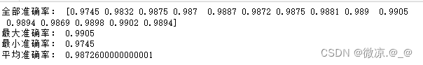
查看验证集准确率:
# 查看结果:
print("全部准确率:",val_eopch_accuracy)
print("最大准确率:",val_eopch_accuracy.max())
print("最小准确率:",val_eopch_accuracy.min())
print("平均准确率:",val_eopch_accuracy.mean())
损失变化可视化:
plt.figure(figsize=(8,8))
x_t = range(len(train_batch_loss[::50]))
y_t = train_batch_loss[::50]

x_v = range(len(val_batch_loss[::10]))
y_v = val_batch_loss[::10]
plt.plot(x_t,y_t,c="r",label="train")
plt.plot(x_v,y_v,c="g",label="val")
plt.title("loss change")
plt.legend()
plt.show()


 876
876


 被折叠的 条评论
为什么被折叠?
被折叠的 条评论
为什么被折叠?
 到【灌水乐园】发言


