【计量经济学】时间序列分析笔记（上）

时间序列复习

密码 2022年6月11日-6月13日

额外的参考资料：北大金融时间序列的备课笔记

Chapter 2 Difference Equations and Their Solutions

通解的描述

This solution $y_t=A{\varphi }_1^t$ to the homogeneous equation is called the homogeneous solution.

• If $\left|{\varphi }_1\right|<1$, ==the homogeneous solution converges to zero as $t\to \infty$.==Convergence is direct if $0<{\varphi }_1<1$ and oscillatory if $-1<{\varphi }_1<0$
• If $\left|{\varphi }_1\right|>1$, the homogeneous solution is divergent. If ${\varphi }_1>1$, the solution approaches $\infty$ as $t$ increases. If ${\varphi }_1<-1$, the solution oscillates explosively.
• If ${\varphi }_1=1$, any arbitrary constant $A$ satisfies the homogeneous equation and $y_t=y_{t-1}$. If ${\varphi }_1=-1,y_t=A$ for even values of $t$ and $y_t=-A$ for odd values of $t$, and $y_t=-y_{t-1}$.

odd:奇数 even: 偶数

差分方程的求解过程

1. 找到齐次方程并求解
2. 找到特解
3. 得到通解
4. 代入初始条件，得到一些常数参数的取值（如果有的话）

lag operators

For $|a|<1$, the infinite sum
$$\left(1+aL+a^2{L}^2+a^3{L}^3+\cdots \right)y_t=\frac{y_t}{1-aL}$$
可以通过等比数列的求和公式得到

可以使用lag来求解差分方程

It is straightforward to use lag operators to solve linear difference equations. If $\left|{\varphi }_1\right|<1$, we obtain
$$\begin{array}{rl}{y}_t& ={\left(1-{\varphi }_{1}L\right)}^{-1}\left({\varphi }_0+x_t\right)=\left(1+{\varphi }_{1}L+{\varphi }_1^2{L}^2+\cdots \right)\left({\varphi }_0+x_t\right)\\ & =\frac{{\varphi }_0}{1-{\varphi }_1}+\sum _{j=0}^{\infty }{\varphi }_1^j{x}_{t-j}\end{array}$$

特征方程

characteristic equation and inverse characteristic equation

求解
$$A{\alpha }^t={\varphi }_{1}A{\alpha }^{t-1}+{\varphi }_{2}A{\alpha }^{t-2}\Rightarrow \underset{\text{characteristic equation }}{\underbrace{{\alpha }^2-{\varphi }_1\alpha -{\varphi }_2=0}}$$
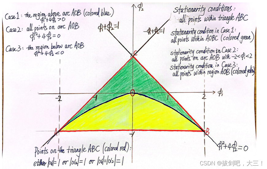
Case 1: If ${\varphi }_1^2+4{\varphi }_2>0,{\alpha }_1,{\alpha }_2=\frac{{\varphi }_1\pm \sqrt{{\varphi }_1^2+4{\varphi }_2}}{2}$
$$y_t=A_1{\alpha }_1^t+A_2{\alpha }_2^t$$
Case 2: If ${\varphi }_1^2+4{\varphi }_2=0,{\alpha }_1={\alpha }_2=\frac{{\varphi }_1}{2}$
$$y_t=A_1{\left(\frac{{\varphi }_1}{2}\right)}^t+A_{2}t{\left(\frac{{\varphi }_1}{2}\right)}^t$$
Case 3: If ${\varphi }_1^2+4{\varphi }_2<0,{\alpha }_1,{\alpha }_2=\frac{{\varphi }_1\pm i\sqrt{-{\varphi }_1^2-4{\varphi }_2}}{2}$.
$$\begin{array}{rl}& {\alpha }_1=\frac{{\varphi }_1+i\sqrt{-{\varphi }_1^2-4{\varphi }_2}}{2}=r(\cos \theta +i\sin \theta )\\ & {\alpha }_2=\frac{{\varphi }_1-i\sqrt{-{\varphi }_1^2-4{\varphi }_2}}{2}=r(\cos \theta -i\sin \theta )\end{array}$$
where $r=\sqrt{-{\varphi }_2}$ is the modulus of ${\alpha }_1$ and ${\alpha }_2$,

and $\theta =\arccos \left(\frac{{\varphi }_1}{2\sqrt{-{\varphi }_2}}\right)$ is the argument of ${\alpha }_1$ and ${\alpha }_2$.
$$y_t=A_1{\alpha }_1^t+A_2{\alpha }_2^t\equiv B_1{r}^t\cos \left(\theta t+B_2\right)$$

stability conditions

Stability requires that all characteristic roots (defined in Eq. (10)) lie within the unit circle, i.e. $\left|{\alpha }_j\right|<1$ for all $j$.

• a necessary condition for stability : ${\sum }_{j=1}^p{\varphi }_j<1$.
• a sufficient condition for stability : ${\sum }_{j=1}^p\left|{\varphi }_j\right|<1$.
• At least one characteristic root equals unity if

$$\sum _{j=1}^p{\varphi }_j=1$$

Chapter 3 Univariate Time Series

介绍MA(q), AR§, ARMA(p,q)

white noise

{ ϵ t } \left\{\epsilon_{t}\right\} {ϵt​} is called a white noise process if for all $t$
$$\begin{array}{rl}E\left({ϵ}_t\right)& =0\text{ mean zero }\\ E\left({ϵ}_t^2\right)& =\mathrm{var}\left({ϵ}_t\right)={\sigma }^2\text{ variance }{\sigma }^2\\ E\left({ϵ}_t{ϵ}_{\tau }\right)& =\mathrm{cov}\left({ϵ}_t,{ϵ}_{\tau }\right)=0,\text{ for all }\tau \ne t\text{ uncorrelated across time }\end{array}$$
If in addition, { ϵ t } \left\{\epsilon_{t}\right\} {ϵt​} is independent across time, then it is called an independent white noise process.
If furthermore, ${ϵ}_t\sim N\left(0,{\sigma }^2\right)$, then we have the Gaussian white noise process.

stationarity

Strict or strong stationarity :

• distributions are time-invariant. This is a very strong condition that is hard to verify empirically.
• 均值和方差不一定有限

Weak stationarity( covariance stationary) :

• first 2 moments are time-invariant. In this course, we are mainly concerned with weakly stationary series.

A stochastic process { y t } \left\{y_{t}\right\} {yt​} having a finite mean and variance is covariance stationary (weakly stationary) if
(1) Mean (or expectation) is the same for each period:
$$E\left(y_t\right)=\mu \text{ for all }t$$
(2) Variance (variability) is the same for each period:
$$\mathrm{var}\left(y_t\right)=E\left[{\left(y_t-\mu \right)}^2\right]={\sigma }_y^2\text{ for all }t$$
(3) Lag-k autocovariance :
$${\gamma }_k=\mathrm{cov}\left(y_t,y_{t-k}\right)=E\left[\left(y_t-\mu \right)\left(y_{t-k}-\mu \right)\right]foralltandanyk$$
与t无关，都是常数

Lag-k autocorrelation (or serial correlation)
$${\rho }_k\equiv \frac{\mathrm{cov}\left(y_t,y_{t-k}\right)}{\mathrm{var}\left(y_t\right)}=\frac{{\gamma }_k}{{\gamma }_0}$$
在多元模型行中，自协方差是指$y_t$和其滞后项之间的协方差，而协方差是指一个序列和另一个序列之间的协方差。在一元时间序列模型中不会产生歧义。

MA(q) models

$$x_t=\mu +\sum _{j=0}^q{\beta }_j{ϵ}_{t-j}MA(q)models$$

${\beta }_0$ is always set to be unity for normalization.

使用stationarity的定义可以得到MA(q)是stationarity的

绝对值求和收敛那么平方和也收敛

AR§ models

$$y_t={\varphi }_0+\sum _{j=1}^p{\varphi }_j{y}_{t-j}+{ϵ}_t,\mathrm{A}\mathrm{R}(\mathrm{p})\text{ model. }$$

Without initial conditions, the general solution to Eq.(6) is:
$$y_t=A{\varphi }_1^t+\frac{{\varphi }_0}{1-{\varphi }_1}+\sum _{j=0}^{\infty }{\varphi }_1^j{ϵ}_{t-j},\text{ if }\left|{\varphi }_1\right|<1.$$

• The characteristic root ${\varphi }_1$ must be less than unity in absolute value.
• The homogeneous solution $A{\varphi }_1^t$ must be zero. Either the sequence must have started infinitely far in the past (so that ${\varphi }_1^t\approx 0$ ) or the process must always be in equilibrium (so that $A=0)$

或者

Stationarity conditions for AR§ processes

• $\left|{\alpha }_j\right|<1$ for all $j=1,\cdots ,p$.
• The homogeneous solution must be zero. Either the sequence must have started infinitely far in the past or the process must always be in equilibrium (so that the arbitrary constants are zero).

ARMA(p,q) models

$$y_t={\varphi }_0+\sum _{j=1}^p{\varphi }_j{y}_{t-j}+\sum _{j=0}^q{\beta }_j{ϵ}_{t-j},\mathrm{ARMA}(\mathrm{p},\mathrm{q})\text{ model. }$$

特解：
$$y_t=c+\sum _{j=0}^{\infty }{c}_j{ϵ}_{t-j}$$

特解+齐次方程的通解即可得到ARMA(p,q)的解

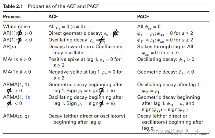
ACF

• The plot of==${\gamma }_k$==against $k$ is called the autocovariance function.

• ACF: The plot of==${\rho }_k$== against $k$ is called the autocorrelation function (ACF) or correlogram.

$${\rho }_k\equiv \frac{\mathrm{cov}\left(y_t,y_{t-k}\right)}{\mathrm{var}\left(y_t\right)}=\frac{{\gamma }_k}{{\gamma }_0}$$

Yule-Walker equations

用于分析ACF

The first $p$ Yule-Walker equations determine the initial conditions.

• The key point is that { γ k } \left\{\gamma_{k}\right\} {γk​} and { ρ k } \left\{\rho_{k}\right\} {ρk​} eventually will satisfy the homogeneous equation of this $AR(p)$ process.
• ACF should converge to zero geometrically if the series is stationary.

一定要注意每一项之间的关系，不要漏掉

Form the Yule-Walker equations :
$$\begin{array}{rl}E\left(y_t{y}_t\right)& ={\varphi }_{1}E\left(y_{t-1}{y}_t\right)+{\varphi }_{2}E\left(y_{t-2}{y}_t\right)+E\left({ϵ}_t{y}_t\right)\\ & \Rightarrow {\gamma }_0={\varphi }_1{\gamma }_1+{\varphi }_2{\gamma }_2+{\sigma }^2\\ E\left(y_t{y}_{t-1}\right)=& {\varphi }_{1}E\left(y_{t-1}{y}_{t-1}\right)+{\varphi }_{2}E\left(y_{t-2}{y}_{t-1}\right)+E\left({ϵ}_t{y}_{t-1}\right)\\ \Rightarrow & {\gamma }_1={\varphi }_1{\gamma }_0+{\varphi }_2{\gamma }_1\\ E\left(y_t{y}_{t-k}\right)=& {\varphi }_{1}E\left(y_{t-1}{y}_{t-k}\right)+{\varphi }_{2}E\left(y_{t-2}{y}_{t-k}\right)+E\left({ϵ}_t{y}_{t-k}\right)\\ \Rightarrow & {\gamma }_k={\varphi }_1{\gamma }_{k-1}+{\varphi }_2{\gamma }_{k-2}\text{ for }k\ge 2\end{array}$$

partial autocorrelation function(PACF)

$$\begin{array}{rl}{y}_t& ={\varphi }_{1,0}+{\varphi }_{1,1}{y}_{t-1}+e_{1t}\\ y_t& ={\varphi }_{2,0}+{\varphi }_{2,1}{y}_{t-1}+{\varphi }_{2,2}{y}_{t-2}+e_{2t}\\ y_t& ={\varphi }_{3,0}+{\varphi }_{3,1}{y}_{t-1}+{\varphi }_{3,2}{y}_{t-2}+{\varphi }_{3,3}{y}_{t-3}+e_{3t}\\ y_t& ={\varphi }_{4,0}+{\varphi }_{4,1}{y}_{t-1}+{\varphi }_{4,2}{y}_{t-2}+{\varphi }_{4,3}{y}_{t-3}+{\varphi }_{4,4}{y}_{t-4}+e_{4t}\\ & ⋮\end{array}$$

{ ϕ k , k , k ≥ 1 } \left\{\phi_{k, k}, k \geq 1\right\} {ϕk,k​,k≥1} is the partial autocorrelation function.

• $e_{it}$ 不一定是白噪音
• $e_{it}$ 与$y_{t-1},y_{t-2},\cdots$ 无关

我们可以利用Yule-Walker方程从ACF中推导出PACF。
$$\begin{array}{rl}E\left(y_t{y}_{t-1}\right)& ={\varphi }_{2,1}E\left(y_{t-1}{y}_{t-1}\right)+{\varphi }_{2,2}E\left(y_{t-2}{y}_{t-1}\right)+E\left(y_{t-1}{e}_{2t}\right)\\ & \Rightarrow {\gamma }_1={\varphi }_{2,1}{\gamma }_0+{\varphi }_{2,2}{\gamma }_1\Rightarrow {\rho }_1={\varphi }_{2,1}+{\varphi }_{2,2}{\rho }_1\\ E\left(y_t{y}_{t-2}\right)& ={\varphi }_{2,1}E\left(y_{t-1}{y}_{t-2}\right)+{\varphi }_{2,2}E\left(y_{t-2}{y}_{t-2}\right)+E\left(y_{t-2}{e}_{2t}\right)\\ & \Rightarrow {\gamma }_2={\varphi }_{2,1}{\gamma }_1+{\varphi }_{2,2}{\gamma }_0\Rightarrow {\rho }_2={\varphi }_{2,1}{\rho }_1+{\varphi }_{2,2}\end{array}$$
Thus ${\varphi }_{2,2}=\frac{{\rho }_2-{\rho }_1^2}{1-{\rho }_1^2}$. For any ${\varphi }_{k,k},k\ge 1$, the similar procedure works.

$$y_t={\varphi }_0+\sum _{j=1}^p{\varphi }_j{y}_{t-j}+\sum _{j=0}^q{\beta }_j{ϵ}_{t-j},\mathrm{ARMA}(\mathrm{p},\mathrm{q})\text{ model. }$$

• 假设一个序列是平稳的，我们可以使用样本均值、方差、ACF和PACF来估计实际数据生成过程的参数。

• 样本ACF和样本PACF可以与各种理论函数进行比较，以帮助识别数据生成过程的实际性质。

Sample mean : $\bar{y}=\frac{{\sum }_{t=1}^T{y}_t}{T}$
Sample variance $:{\hat{\sigma }}_y^2=\frac{{\sum }_{t=1}^T{\left(y_t-\bar{y}\right)}^2}{T}$.
Lag-k sample autocorrelation:
$${\hat{\rho }}_k=\frac{{\sum }_{t=k+1}^T\left(y_t-\bar{y}\right)\left(y_{t-k}-\bar{y}\right)}{{\sum }_{t=1}^T{\left(y_t-\bar{y}\right)}^2}k\ge 1.$$
The statistics { ρ ^ 1 , ρ ^ 2 , … } \left\{\widehat{\rho}_{1}, \widehat{\rho}_{2}, \ldots\right\} {ρ ​1​,ρ ​2​,…} are called the sample ACF of { y t } \left\{y_{t}\right\} {yt​}

ARMA(p,q)阶数的识别

t test

检验ACF的，即判断q有几阶

For a given positive integer $k$, test $H_0:{\rho }_k=0$ against $H_1:{\rho }_k\ne 0$

• If { y t } \left\{y_{t}\right\} {yt​} is a stationary Gaussian series satisfying ${\rho }_j=0$ for $j\ge k$ (i.e., if { y t } \left\{y_{t}\right\} {yt​} is an $\mathrm{M}\mathrm{A}(\mathrm{k}-1)$ with normally distributed { ϵ t } \left\{\epsilon_{t}\right\} {ϵt​} ), then ${\hat{\rho }}_k$ is asymptotically normal with mean zero and variance $\frac{1+2{\sum }_{j=1}^{k-1}{\rho }_j^2}{T}$. Therefore, the test statistic is
  $$\mathrm{t}\text{ ratio }=\frac{{\hat{\rho }}_k}{\sqrt{\left(1+2{\sum }_{j=1}^{k-1}{\hat{\rho }}_j^2\right)/T}}\stackrel{\mathcal{D}}{⟶}\mathcal{N}(0,1),\text{ as }T\to \infty$$
  ​ where $\stackrel{\mathcal{D}}{⟶}$ denotes “converge in distribution”.

• If { y t } \left\{y_{t}\right\} {yt​} is an i.i.d. sequence satisfying $\mathrm{var}\left(y_t\right)<\infty$ (i.e., if { y t } \left\{y_{t}\right\} {yt​} is an i.i.d. $\mathrm{M}\mathrm{A}(0))$, then ${\hat{\rho }}_k$ is asymptotically normal with mean zero and variance $\frac{1}{T}$ for any $k\ge 1$. Thus $t$ ratio $=\frac{{\hat{\rho }}_k}{\sqrt{1/T}}\stackrel{\mathcal{D}}{⟶}\mathcal{N}(0,1)$, for sufficiently large $T$.

• { ρ ^ 1 , ρ ^ 2 , … } \left\{\widehat{\rho}_{1}, \widehat{\rho}_{2}, \ldots\right\} {ρ ​1​,ρ ​2​,…} will be calculated along with the acceptance intervals (significance level $=5\%$ ) under this i.i.d. assumption, once you put the data into Eviews or MATLAB.

检验过程

t>|1.96|拒绝 t<|1.96|接受

1. $H_0:{\rho }_1=0H_1:q\ge 1$. $t=\frac{\widehat{\rho}_{k}}{\sqrt{1 / T}} $
2. 拒绝原假设，则继续检验
3. $H_0:{\rho }_2=0H_1:q\ge 2$. $t\text{ ratio }=\frac{{\hat{\rho }}_k}{\sqrt{\left(1+2{\sum }_{j=1}^{k-1}{\hat{\rho }}_j^2\right)/T}}$
4. 直到接受原假设，此时可与得到q的阶数

Joint Test (Ljung-Box Q-statistics)

联合检验ACF，判断q值

• Significance test for a group of autocorrelations $H_0:{\rho }_I=\cdots ={\rho }_m=0$ against $H_1:{\rho }_i\ne 0$ for some $1\le i\le m$
• Under the assumption that { y t } \left\{y_{t}\right\} {yt​} is an i.i.d. sequence with certain moment conditions
  $$Q(m)=T(T+2)\sum _{k=1}^m\frac{{\hat{\rho }}_k^2}{T-k}\stackrel{\mathcal{D}}{⟶}{\chi }_m^2$$
• Decision rule : reject $H_0$ if $Q(m)>{\chi }_m^2(\alpha )$, where ${\chi }_m^2(\alpha )$ denotes the $100(1-\alpha )$ th percentile of a chi-squared distribution with $m$ degrees of freedom.

Q检验也可以判断残差是否为白噪音，但自由度会减小
$$Q(m)=T(T+2)\sum _{k=1}^m\frac{{\tilde{\rho }}_k^2}{T-k}\stackrel{\mathcal{D}}{⟶}{\chi }_{m-g}^2,$$
where ${\tilde{\rho }}_k$ is the sample ACF of estimation residuals, and $g$ denotes 模型中固定的常数的个数

PACF可以帮助识别P

对于平稳的AR§模型

${\hat{\varphi }}_{k,k}$ converges to ${\varphi }_{k,k}$ in probability as the sample size $T$ goes to infinity.

• ${\varphi }_{p,p}={\varphi }_p$
• ${\varphi }_{k,k}=0$ for $k>p$.
  For $k>p,{\hat{\varphi }}_{k,k}$ is asymptotically normal with mean zero and variance $\frac{1}{T}$

t>|1.96|拒绝 t<|1.96|接受

1. $H_0:{\rho }_1=0H_1:p\ge 1$. $|PACF|>\frac{ 1.96}{\sqrt{1 / T}} $ 拒绝原假设
2. 拒绝原假设，则继续检验
3. $H_0:{\rho }_2=0H_1:p\ge 2$. $|PACF|>\frac{ 1.96}{\sqrt{1 / T}} $ 拒绝原假设
4. 直到接受原假设，此时可与得到q的阶数

Criteria: AIC, BIC

自由度和残差的一些trade off

• Akaike information criterion (AIC):
  $$AIC(I)=\underset{\text{goodness of fit }}{\underbrace{\log \left({\tilde{\sigma }}_l^2\right)}}+\underset{\text{penalty function }}{\underbrace{\frac{2I}{T}}}$$
  where $/$ is the number of parameters estimated and ${\tilde{\sigma }}_I^2=\frac{SSR}{T}$.

• Bayesian information criterion (BIC) or Schwarz information criterion $(\mathrm{S}\mathrm{B}\mathrm{C},\mathrm{S}\mathrm{I}\mathrm{C})$ :
  $$BIC(I)=\underset{\text{goodness of fit }}{\underbrace{\log \left({\tilde{\sigma }}_l^2\right)}}+\underset{\text{penalty function }}{\underbrace{\frac{\log (T)}{T}}}$$
  Choose the model with minimum $\mathrm{A}\mathrm{I}\mathrm{C}$ or $\mathrm{B}\mathrm{I}\mathrm{C}$.

• BIC适用于大样本。BIC将渐近地提供正确的模型，而AIC则倾向于选择一个过参数化的模型。

• 在小样本中，AIC比BIC工作得更好。在BIC的背景下，来自给定总体中不同样本的选定模型顺序的平均变化将大于AIC。

如果他们建议不同的模型，应该选择哪个IC？

• 由于BIC选择了更简洁的模型，因此您应该检查以确定残差是否显示为白噪声。
• 由于AIC可以选择一个过度参数化的模型，因此所有系数的t-统计量在传统水平上都应该是显著的。
• 可能无法找到一个明显占优于所有其他模型的模型

检验 ： 残差是否为白噪音 预测未来的数据

Box-Jenkins Approach

Box and Jenkins $(1970,1976)$ popularized a three-stage method to estimate an ARMA model in a systematic manner.

1. Identification

2. Estimation

3. Model diagnostic checking

4. Identification

• First of all, one might visually examine the time plot of the series, sample ACF and sample PACF. A comparison of the sample ACF and PACF to those of various theoretical ARMA processes may suggest several candidate models.
• Model specification: AIC, BIC.

Parsimony简洁原则

• Similar processes can be approximated by very different models.
• Common factor problem.
• Each coefficient is significantly different from zero at the conventional level.

2. Estimation

Estimation can be done using least squares or maximum likelihood depending on the model.

• AR models : least squares method or maximum likelihood method
• MA and ARMA models : maximum likelihood method

残差平方和最小和极大似然估计

Stationarity and Invertibility

• t-stats, ACF, Q-stats, $\cdots$ all assume that the process is stationary.
• Be suspicious of implied roots near the unit circle.
• Invertibility implies the model has an AR representation.
  • No unit root in MA part of the model. 在MA模型中无单位根
  • ARMA(p，q)过程的可逆性条件完全由它的MA部分决定。

极大似然估计?

待完善。。。

3. Model diagnostic checking

• Residual diagnostics :
  • Plot residuals : look for outliers and periods of poor fit.
  • Residuals should be serially uncorrelated : examine ACF, PACF, Q-stats of residuals.残差要序列不相关
• Divide sample into subperiods 样本内预测，看拟合效果
• Out-of-sample forecasts 样本外预测

预测

条件均值（期望）

This result is really quite general: for any stationary ARMA model, the conditional forecast of $y_{t+j}$ converges to the unconditional mean as $j\to \infty$.
$$e_t(j)=y_{t+j}-E_t{y}_{t+j}$$
The $95\%$ confidence interval for the $j$-step ahead forecast is :
$$\left[E_t{y}_{t+j}-1.96\sqrt{\mathrm{var}\left(e_t(j)\right)},E_t{y}_{t+j}+1.96\sqrt{\mathrm{var}\left(e_t(j)\right)}\right]\text{. }$$

test whether a forecast is accurate or not

We want the forecast errors to be small!

If there are $\mathrm{H}$ observations in the holdback periods, and { e j } j = 1 H \left\{e_{j}\right\}_{j=1}^{H} {ej​}j=1H​ are the forecast errors from the candidate model :

• Mean squared prediction error: MSPE $=\frac{1}{H}{\sum }_{j=1}^H{e}_j^2$. It is also called mean squared error (MSE).
• Mean absolute error: $\mathrm{M}\mathrm{A}\mathrm{E}=\frac{1}{H}{\sum }_{j=1}^H\left|e_j\right|$.
• Mean absolute percentage error: MAPE $=\frac{1}{H}{\sum }_{j=1}^H\left|\frac{e_j}{y_{T+j}}\right|\cdot 100$.

Many researchers would select the model with the smallest MSPE (or MAE, MAPE).

Diebold-Mariano Test

• Let the loss from a forecast error in period $j$ be denoted by $g\left(e_j\right)$. In the typical case of mean squared errors, the loss is $e_j^2$
• We can write the differential loss in period $j$ from using model 1 versus model 2 as $d_j=g\left(e_{1j}\right)-g\left(e_{2j}\right)$. The mean loss can be obtained as
  $$\bar{d}=\frac{1}{H}\sum _{j=1}^H\left[g\left(e_{1j}\right)-g\left(e_{2j}\right)\right]$$
• Under the null hypothesis of equal forecast accuracy,
  • $H_0:E(\bar{d})=E\left(d_j\right)=0$
  • $H_1:E(\bar{d})>0?E(\bar{d})<0?$ （模型2更好，模型1更好）

Under fairly weak conditions, the central limit theorem implies that $\bar{d}\stackrel{\mathcal{D}}{⟶}\mathcal{N}(0,\mathrm{var}(\bar{d}))$, as $H\to \infty$, under the null hypothesis.

• If the { d j } \left\{d_{j}\right\} {dj​} series is serially uncorrelated with a sample variance of $\hat{\gamma }$, 若序列无关the estimator of $\mathrm{var}(\bar{d})$ is simply $\frac{\hat{\gamma }}{H-1}$. The expression
  $$\frac{\bar{d}}{\sqrt{\hat{\gamma }/(H-1)}}\stackrel{\mathcal{D}}{⟶}\mathcal{N}(0,1),\text{ as }H\to \infty ,$$
  ​ under the null hypothesis.

• If the { d j } \left\{d_{j}\right\} {dj​} series is serially correlated,若序列相关 there is a very large literature on the best way to estimate $\mathrm{var}(\bar{d})$ in the presence of serial correlation (e.g., the Newey-West estimator of the variance proposed in Newey and West $(1987))$.
  $$\frac{\bar{d}}{\sqrt{\widehat{\mathrm{var}(\bar{d})}}}\stackrel{\mathcal{D}}{⟶}\mathcal{N}(0,1),\text{ as }H\to \infty$$
  ​ under the null hypothesis, where $\widehat{\mathrm{var}(\bar{d})}$ is an appropriate estimator of $\mathrm{var}(\bar{d})$.

双边检验：1.96

单边检验：1.645

$H_1: \quad E(\bar{d})>0 ? $ 模型二更好1.645

$E(\bar{d})<0?$ 模型一更好-1.645

time series with trend

1. 做差分去趋势化(log difference)
2. 直接回归方程

周期性或季节性ARMA model

拟合模型应同时考虑数据中的季节模式和非季节模式。

Chapter 4 Modeling Volatility

the volatility equation:
$${\sigma }_t^2=\mathrm{var}\left(y_t\mid {\mathcal{F}}_{t-1}\right)=\mathrm{var}\left({ϵ}_t\mid {\mathcal{F}}_{t-1}\right)$$

• Volatility ${\sigma }_t$ : the conditional standard deviation of $y_t$ based on a past information set ${\mathcal{F}}_{t-1}$.

ARCH(q) 自回归条件异方差

A natural idea is to model ${ϵ}_t^2$ using an $AR(q)$ process:
$$\begin{array}{rl}{ϵ}_t^2& ={\alpha }_0+{\alpha }_1{ϵ}_{t-1}^2+\cdots +{\alpha }_q{ϵ}_{t-q}^2+{\eta }_t\\ \Rightarrow {\sigma }_t^2& ={\alpha }_0+{\alpha }_1{ϵ}_{t-1}^2+\cdots +{\alpha }_q{ϵ}_{t-q}^2\end{array}$$
Eq. is called an autoregressive conditional heteroskedasticity $(\mathbf{A}\mathbf{R}\mathbf{C}\mathbf{H})$ model of order $q$.

ARCH (q) model
$$\begin{array}{rl}{y}_t& =E\left(y_t\mid {\mathcal{F}}_{t-1}\right)+{ϵ}_t,{ϵ}_t={\sigma }_t{v}_t\\ {\sigma }_t^2& ={\alpha }_0+{\alpha }_1{ϵ}_{t-1}^2+\cdots +{\alpha }_q{ϵ}_{t-q}^2\end{array}$$

• This is an ARCH (q) model.
• ${\alpha }_0>0$, and ${\alpha }_i\ge 0$ for $i>0$ for positiveness.
• ${\sum }_{i=1}^q{\alpha }_i<1$ for stationarity.
• { v t } \left\{v_{t}\right\} {vt​} is a sequence of i.i.d.r.v. with mean 0 and variance 1 .

协方差Cov( , )反映的是线性相关关系

Corr( , )表示是否相关 独立是p(xy)=p(x)p(y)

善用全期望公式
$$\begin{array}{rl}E\left({ϵ}_t\right)& =E\left[E\left({ϵ}_t\mid {\mathcal{F}}_{t-1}\right)\right]=0\\ E\left({ϵ}_t{ϵ}_{t-j}\right)& =E\left[E\left({ϵ}_t{ϵ}_{t-j}\mid {\mathcal{F}}_{t-1}\right)\right]=E\left[{ϵ}_{t-j}E\left({ϵ}_t\mid {\mathcal{F}}_{t-1}\right)\right]=0j\ge 1\end{array}$$

${ϵ}_t^2$

Assuming stationarity $\left({\alpha }_1+\cdots +{\alpha }_q<1\right)$
$$\begin{array}{rl}\mathrm{var}\left({ϵ}_t\right)& =E\left({ϵ}_t^2\right)=E\left[E\left({ϵ}_t^2\mid {\mathcal{F}}_{t-1}\right)\right]=E\left({\sigma }_t^2\right)\\ & ={\alpha }_0+{\alpha }_{1}E\left({ϵ}_{t-1}^2\right)+\cdots +{\alpha }_{q}E\left({ϵ}_{t-q}^2\right)\end{array}$$
which implies that
$$\mathrm{var}\left({ϵ}_t\right)=E\left({\sigma }_t^2\right)=\frac{{\alpha }_0}{1-{\alpha }_1-\cdots -{\alpha }_q}$$
The error { ϵ t } \left\{\epsilon_{t}\right\} {ϵt​} is uncorrelated and stationary with mean zero and constant unconditional variance (with constraints to $\mathrm{A}\mathrm{R}\mathrm{C}\mathrm{H}$ parameters).

${ϵ}_t^2$ 是一个白噪音，uncorrelated, but dependent. 非线性相关关系

ARCH Model 可以描述序列的平稳性和波动性

Heavy tails

long tail / fat tail/ heavy tail

• Kurtosis of a random variable $y$ is defined to be $\frac{E\left[(y-E(y){)}^4\right]}{[\mathrm{var}(y){]}^2}$. For example,
• the kurtosis of a normal distribution is $3.$
• the kurtosis of a student’s $\mathrm{t}$ distribution with $\nu$ degrees of freedom is $\frac{6}{\nu -4}+3$, for $\nu >4$.
• Kurtosis identifies whether the tails of a given distribution contain extreme values.
• Excess kurtosis=kurtosis-3 defines how heavily the tails of a distribution differ from the tails of a normal distribution.

ARCH heavy tail

Advantages

• Simplicity
• $\mathrm{A}\mathrm{R}\mathrm{C}\mathrm{H}$ can model the volatility clustering effect since the conditional variance is autoregressive. Such models can be used to forecast volatility.
• Heavy tails (high kurtosis)

Weaknesses

• Symmetric between positive & negative prior shocks
• Restrictive on parameter space

Idea : $\mathrm{A}\mathrm{R}\mathrm{C}\mathrm{H}$ is like an $\mathrm{A}\mathrm{R}$ model for volatility. $\mathrm{G}\mathrm{A}\mathrm{R}\mathrm{C}\mathrm{H}$ is like an ARMA model for volatility.

$GARCH(p,q)$ model :

$$\begin{array}{rl}{y}_t& =E\left(y_t\mid {\mathcal{F}}_{t-1}\right)+{ϵ}_t{ϵ}_t={\sigma }_t{v}_t\\ {\sigma }_t^2& ={\alpha }_0+\sum _{i=1}^q{\alpha }_i{ϵ}_{t-i}^2+\sum _{j=1}^p{\beta }_j{\sigma }_{t-j}^2\end{array}$$

• ${\alpha }_0>0$, and ${\alpha }_i\ge 0,{\beta }_j\ge 0$ for $i,j>0$ ensure positiveness.
• ${\sum }_{i=1}^{\max (p,q)}\left({\alpha }_i+{\beta }_i\right)<1$ ensures stationarity.（证明如下）
• { v t } \left\{v_{t}\right\} {vt​} is a sequence of i.i.d. r.v. with mean 0 and variance 1 .

Re-parameterization :
Let η t = ϵ t 2 − σ t 2 . { η t } \eta_{t}=\epsilon_{t}^{2}-\sigma_{t}^{2} .\left\{\eta_{t}\right\} ηt​=ϵt2​−σt2​.{ηt​} are uncorrelated series. The $\mathrm{G}\mathrm{A}\mathrm{R}\mathrm{C}\mathrm{H}$ model becomes
$${ϵ}_t^2={\alpha }_0+\sum _{i=1}^{\max (p,q)}\left({\alpha }_i+{\beta }_i\right){ϵ}_{t-i}^2+{\eta }_t-\sum _{j=1}^p{\beta }_j{\eta }_{t-j}$$
This is an ARMA form for the squared series ${ϵ}_t^2$.

The error { ϵ t } \left\{\epsilon_{t}\right\} {ϵt​} is uncorrelated and stationary with mean zero and finite unconditional variance,
$$\begin{array}{rl}E\left({ϵ}_t\mid {\mathcal{F}}_{t-1}\right)& =0,E\left({ϵ}_t\right)=0,E\left({ϵ}_t{ϵ}_{t-j}\right)=0j\ge 1\\ \mathrm{var}\left({ϵ}_t\right)& =E\left({ϵ}_t^2\right)=\frac{{\alpha }_0}{1-\left({\sum }_{i=1}^m{\alpha }_i\right)-\left({\sum }_{j=1}^s{\beta }_j\right)}\end{array}$$
provided that ${\sum }_{i=1}^{\max (m,s)}\left({\alpha }_i+{\beta }_i\right)<1$

GARCH heavy tails

一般来说，一个GARCH（1,1）模型将足以捕获数据中的波动性聚类。

除了ARCH,GARCH，还有其他的包含过去信息的形式的模型

Identification of $\mathrm{A}\mathrm{R}\mathrm{C}\mathrm{H}$ and GARCH Models

1. Modeling the mean equation and testing for $\mathrm{A}\mathrm{R}\mathrm{C}\mathrm{H}$ effects.
   • $H_0$ : no $\mathrm{A}\mathrm{R}\mathrm{C}\mathrm{H}$ effects versus $H_1:\mathrm{A}\mathrm{R}\mathrm{C}\mathrm{H}$ effects.
   • Use Q-statistics of squared residuals $\left\{{\widehat{ϵ}}_t^2\right\}$ or LM test.
2. Order determination :
   • PACF of the squared residuals ${\widehat{ϵ}}_t^2$ gives useful information about the ARCH order $q$ (see Eq.(2)); 、
   • to identify GARCH models, we use information criteria.

Testing for ARCH Effects

类似于AR model的检验

Ljung-Box statistics

Consider testing $H_0:($ No $\mathrm{A}\mathrm{R}\mathrm{C}\mathrm{H}){\alpha }_1={\alpha }_2=\cdots ={\alpha }_q=0$ against $H_1:(\mathrm{A}\mathrm{R}\mathrm{C}\mathrm{H})$ at least one ${\alpha }_i\ne 0$

• Step 1 : Compute residuals { ϵ t ^ } \left\{\hat{\epsilon_{t}}\right\} {ϵt​^​} from mean equation regression.
• Step 2 : Apply the usual Ljung-Box statistics $Q(m)$ to $\left\{{\widehat{ϵ}}_t^2\right\}$ series.
• View/Residual Diagnostics : Correlogram Squared Residuals

Engle derived a simple LM test :

• Step 1: Compute residuals { ϵ t ^ } \left\{\hat{\epsilon_{t}}\right\} {ϵt​^​} from mean equation regression.

• Step 2 : Estimate auxiliary regression
  $${\widehat{ϵ}}_t^2={\alpha }_0+{\alpha }_1{\widehat{ϵ}}_{t-1}^2+\cdots +{\alpha }_q{\widehat{ϵ}}_{t-q}^2+{\text{ error }}_t$$
  ​ Obtain $R^2\equiv R_{AUX}^2$ from this regression.

• Step 3 : Form the LM test statistic
  $$L{M}_{ARCH}=T\cdot R_{AUX}^2$$
  ​ where $T=$ sample size from auxiliary regression.

​ Under $H_0$ : (No $\mathrm{A}\mathrm{R}\mathrm{C}\mathrm{H}),L{M}_{ARCH}$ is asymptotically distributed as ${\chi }^2(q)$.

Estimation of ARCH/GARCH Models

由于非线性，所以只能使用极大似然估计

The steps involved in actually estimating an $\mathrm{A}\mathrm{R}\mathrm{C}\mathrm{H}$ or GARCH model are as follows :
(1) Specify the appropriate equations for the mean and the variance - e.g. an $\mathrm{A}\mathrm{R}(1)-\mathrm{G}\mathrm{A}\mathrm{R}\mathrm{C}\mathrm{H}(1,1)$ model:
$$\begin{array}{rl}& y_t={\varphi }_0+{\varphi }_1{y}_{t-1}+{ϵ}_t,{ϵ}_t={\sigma }_t{v}_t,v_t\stackrel{i.i.d}{\sim }\mathcal{N}(0,1),\\ & {\sigma }_t^2={\alpha }_0+{\alpha }_1{ϵ}_{t-1}^2+{\beta }_1{\sigma }_{t-1}^2.\end{array}$$
(2) Specify the log-likelihood function to maximize:
$$L=-\frac{T}{2}\log (2\pi )-\frac{1}{2}\sum _{t=1}^T\log \left({\sigma }_t^2\right)-\frac{1}{2}\sum _{t=1}^T\frac{{\left(y_t-{\varphi }_0-{\varphi }_1{y}_{t-1}\right)}^2}{{\sigma }_t^2}.$$
(3) The computer will maximize the function and give estimates and their standard errors.

Model Checking

For a properly specified $\mathrm{A}\mathrm{R}\mathrm{C}\mathrm{H}/\mathrm{G}\mathrm{A}\mathrm{R}\mathrm{C}\mathrm{H}$ model, the standardized residuals
$${\hat{v}}_t=\frac{{\widehat{ϵ}}_t}{{\hat{\sigma }}_t}$$

• If the mean equation is adequate
  • (i.e. the serial correlation in $y_t$ is completely captured),
  • the residuals { ϵ ^ t } \left\{\widehat{\epsilon}_{t}\right\} {ϵ t​} should behave as a white noise process.
  • Consequently, the standardized residuals { v ^ t } \left\{\widehat{v}_{t}\right\} {v t​} should also behave as a white noise process.
• If the volatility equation is adequate
  • (i.e. the dependence in ${ϵ}_t^2$ is completely captured),
  • the squared standardized residuals $\left\{{\hat{v}}_t^2=\frac{{\widehat{ϵ}}_t^2}{{\hat{\sigma }}_t^2}\right\}$ should be uncorrelated across time.

综上所述

1. { v ^ t } \left\{\widehat{v}_{t}\right\} {v t​} 的ljung-box统计量可以用来检验平均方程的充分性。
2. $\left\{{\hat{v}}_t^2=\frac{{\widehat{ϵ}}_t^2}{{\hat{\sigma }}_t^2}\right\}$ 的Ljung-Box统计量可以用来检验波动率方程的充分性。
3. { v ^ t } \left\{\widehat{v}_{t}\right\} {v t​}的偏度、峰度和QQ图可以用来检验分布假设的有效性。???

heavy tail 是用来干啥的以及以上

Forecasting Variances using ARCH Models

Interval Forecasting

Confidence bands for the 1-step ahead forecast at the forecast origin $\mathrm{t}$

• The conditional distribution of $y_{t+1}$ given the information available at time $t$ is $D\left[E\left(y_{t+1}\mid {\mathcal{F}}_t\right),\mathrm{var}\left(y_{t+1}\mid {\mathcal{F}}_t\right)\right]$, where $D$ depends on the distribution of $v_t$.
• $\mathrm{var}\left(y_{t+1}\mid {\mathcal{F}}_t\right)={\sigma }_{t+1}^2$
• Under normality assumption, 95% confidence interval of the prediction is $\left[E\left(y_{t+1}\mid {\mathcal{F}}_t\right)-1.96{\sigma }_{t+1},E\left(y_{t+1}\mid {\mathcal{F}}_t\right)+1.96{\sigma }_{t+1}\right]$.

real data example 考吗？

1. mean equation
2. test for ARCH effect
3. 根据残差项的平方的 ACF PACF判断是使用ARCH还是GARCH
4. estimate mean equation+ARCH/GARCH
5. Wald test-cofficient
6. 有些系数不显著，简化模型
7. Model checking，同时调整
8. forecast