[Python语言程序设计]Python 课程实验

春天熊

已于 2023-06-15 08:26:26 修改

阅读量1.2k

点赞数 1

分类专栏：武理四年文章标签： Python Numpy Pandas Matplotlib Scipy

于 2022-05-18 16:36:39 首次发布

本文链接：https://blog.csdn.net/weixin_51008866/article/details/124844945

版权

武理四年专栏收录该内容

38 篇文章 117 订阅

订阅专栏

Spring-_-Bear 的 CSDN 博客导航

文章目录

第 1 章 Numpy
第 2 章 Pandas
第 3 章 Matplotlib
第 4 章 Scipy
第 5 章 Scikit-learn
第 6 章常用标准库
第 7 章常用数据结构
附录

第 1 章 Numpy

NumPy（Numerical Python）是 Python 的一种开源的数值计算扩展。这种工具可用来存储和处理大型矩阵，比 Python 自身的嵌套列表（nested list structure）结构要高效的多（该结构也可以用来表示矩阵（matrix）），支持大量的维度数组与矩阵运算，此外也针对数组运算提供大量的数学函数库。

1.1 数组

1.1.1 创建数组

程序源码：

import numpy as np

print('一维数组：', np.array([1, 2, 3, 4, 5]))

print('\n多维数组：')
print(np.array([[1, 2, 3], [4, 5, 6]]))

print('\n全 0 多维数组：')
print(np.zeros([2, 2]))

print('\n全 1 多维数组：')
print(np.ones([2, 2]))

print('\n类对角矩阵：')
print(np.eye(3))

print('\n数据转一维数组：', np.asarray([1, 2, 3, 4, 5]))

print('\n一维等间隔数组：', np.arange(10, 20, 2))

print('\n等距数组：', np.linspace(0, 100, 3))

运行示例：

在这里插入图片描述

1.1.2 数组属性

程序源码：

import numpy as np

arr = np.array([[1, 2], [3, 4], [5, 6]])
print('数组行数：', arr.shape[0])
print('数组行数：', np.size(arr, 0))
print('数组行数：', len(arr))
print('数组元素个数：', arr.size)
print('数组形状：', arr.shape)
print('数组维度：', arr.ndim)

print('\n数组变形：')
print(arr.reshape(2, 3))

arr = np.arange(10)
# arr[start:end:step] start = 0, end = len(arr), step = 1
print('\n上下限步长切片：', arr[2:8:2])
print('上下限切片:', arr[2:8])
print('下限切片:', arr[2:])
print('指定元素:', arr[2])

arr = np.array([[1, 2], [3, 4]])
print('\n布尔判断数组：')
print(arr > 2)
print('条件过滤数组：')
print(arr[arr > 2])

运行示例：

在这里插入图片描述

1.1.3 广播

NumPy 的数组广播（broadcasting）是一种机制，它允许在不同形状的数组之间执行元素级操作。当进行操作的数组形状不完全相同时，NumPy 会根据一定的规则进行自动调整，以使它们具有兼容的形状。这样可以方便地进行数组之间的运算，而无需显式地扩展数组的维度或重复数组的元素。

广播规则如下：

如果两个数组的维度数不相同，NumPy 会在较小的维度前面补 1，直到维度数相同。
如果两个数组在任何维度上的大小不匹配，且其中一个数组的大小为 1，那么可以在该维度上进行广播。
如果两个数组在某个维度上的大小既不相等也不为 1，则会引发 ValueError 错误，表示无法进行广播。

程序源码：

import numpy as np

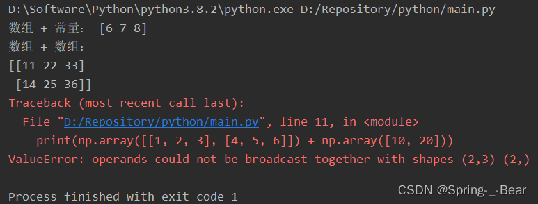
# 示例 1：一个数组与一个标量相加
print('数组 + 常量：', np.array([1, 2, 3]) + 5)

# 示例 2：两个数组相加，在较小的维度前面补 1，直到维度数相同
print('数组 + 数组：')
print(np.array([[1, 2, 3], [4, 5, 6]]) + np.array([10, 20, 30]))

# 示例 3：广播失败，两个数组在某个维度上的大小既不相等也不为 1，则会引发 ValueError 错误
print(np.array([[1, 2, 3], [4, 5, 6]]) + np.array([10, 20]))

运行示例：

在这里插入图片描述

1.1.4 常用函数

flat(): 按照下标取元素，在多维数组中也可以直接取到对应的元素。
np.transpose(): 根据数组的行列索引值对数据进行转换（二维数组默认是转置）。
np.concentrate(): 将多个数组沿指定的轴连接在一起，默认是列。
np.stack(): 沿新轴连接数组序列。它将一系列数组沿着新的维度（轴）进行堆叠，生成一个新的数组。
np.delete(): 删除数组中的指定元素、行或列。它返回一个新的数组，其中删除了指定元素或行/列后的结果。

程序源码：

import numpy as np

# flat(): 按照下标取元素，在多维数组中也可以直接取到对应的元素
arr = np.arange(6).reshape(2, 3)
print('第 1 行:', arr[1])
print('arr.flat[1]:', arr.flat[3])

# np.transpose(): 根据数组的行列索引值对数据进行转换（二维数组默认是转置）
arr = np.array([[1, 2, 3], [4, 5, 6], [7, 8, 9]])
print('\n行列转置：')
print(np.transpose(arr))

# np.concentrate(): 将多个数组沿指定的轴连接在一起，默认是列
arr1 = np.array([[1, 2, 3], [4, 5, 6]])
arr2 = np.array([[7, 8], [9, 10]])
print('\n数组轴连接：')
print(np.concatenate((arr1, arr2), axis=1))

# np.stack(): 沿新轴连接数组序列。它将一系列数组沿着新的维度（轴）进行堆叠，生成一个新的数组
arr1 = np.array([1, 2, 3])
arr2 = np.array([4, 5, 6])
print('\n数组轴堆叠：')
print(np.stack((arr1, arr2), axis=1))

# np.delete(): 删除数组中的指定元素、行或列。它返回一个新的数组，其中删除了指定元素或行/列后的结果
arr = np.array([[1, 2, 3], [4, 5, 6], [7, 8, 9]])
print('\n列元素删除：')
print(np.delete(arr, [0, 2], axis=1))

运行示例：

在这里插入图片描述

1.2 矩阵

1.2.1 创建矩阵

程序源码：

import numpy as np

print('全一矩阵：')
print(np.zeros((2, 2)))
print('全零矩阵：')
print(np.ones((2, 2)))
print('对角矩阵：')
print(np.eye(3))
print('数组转换矩阵：')
print(np.asarray([[1, 2], [3, 4]]))
print('随机矩阵：')
print(np.random.randint(0, 10, (3, 3)))
print('命名空间：')
arr = np.array([1, 2, 3])
print(np.mat(arr))
# matrix 与 asmatrix 的区别在于 asmatrix 处理矩阵或数组时不复制
print(np.asmatrix(arr))
# 类似与 array 与 asarray
print(np.matrix(arr))

运行示例：

在这里插入图片描述

1.2.2 矩阵运算

程序源码：

import numpy as np

arr1 = np.mat([[1], [2], [3]])
arr2 = np.mat([1, 2, 3])
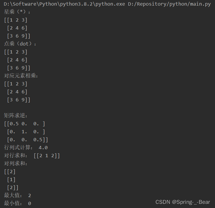
print('星乘（*）：')
print(arr1 * arr2)
print('点乘（dot）：')
print(np.dot(arr1, arr2))
print('对应元素相乘：')
print(np.multiply(arr1, arr2))

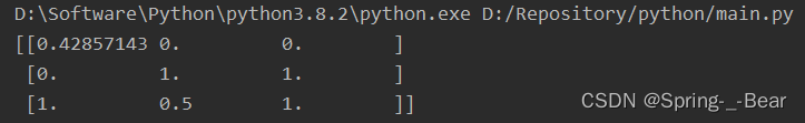
arr = np.matrix([[2, 0, 0], [0, 1, 0], [0, 0, 2]])
print('\n矩阵求逆：')
print(np.linalg.inv(arr))
print('行列式计算：', np.linalg.det(arr))
print('对行求和：', arr.sum(axis=0))
print('对列求和：')
print(arr.sum(axis=1))
print('最大值：', arr.max())
print('最小值：', arr.min())

运行示例：

在这里插入图片描述

1.2.3 矩阵转数组

程序源码：

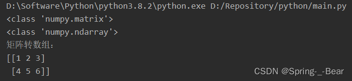
import numpy as np

arr = np.mat([[1, 2, 3], [4, 5, 6]])
print(type(arr))
arr = arr.getA()
print(type(arr))
print('矩阵转数组：')
print(arr)

运行示例：

在这里插入图片描述

1.3 随机模块

1.3.1 简单随机数据

程序源码：

import numpy as np

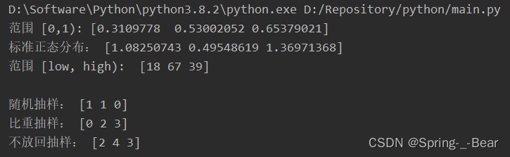
print('范围 [0,1):', np.random.rand(3))
print('标准正态分布：', np.random.randn(3))
print('范围 [low, high): ', np.random.randint(1, 100, 3))

print('\n随机抽样：', np.random.choice(5, 3))
print('比重抽样：', np.random.choice(5, 3, p=[0.1, 0, 0.3, 0.6, 0]))
print('不放回抽样：', np.random.choice(5, 3, replace=False))

运行示例：

在这里插入图片描述

1.3.2 随机排列

程序源码：

import numpy as np

arr = np.array([1, 2, 3, 4, 5])
np.random.shuffle(arr)
print('随机打乱数组：', arr)
print('随机序列：', np.random.permutation([1, 2, 3, 4, 5]))

运行示例：

在这里插入图片描述

1.3.3 常用分布

程序源码：

import numpy as np

# args1: 均值 args2: 标准差 args3: 返回值的维度
print('正态分布：', np.random.normal(0, 0.1, 3))
print('均匀分布：', np.random.uniform(0, 5, 2))
print('泊松分布：', np.random.poisson(5, 2))

运行示例：

在这里插入图片描述

1.4 常用函数

1.4.1 三角函数

程序源码：

import numpy as np
np.set_printoptions(linewidth=1000)

arr = np.array([0, 30, 45, 60, 90])
print('sin:', np.sin(arr / 180 * np.pi))
print('cos:', np.cos(arr / 180 * np.pi))

运行示例：

在这里插入图片描述

1.4.2 四舍五入

程序源码：

import numpy as np

arr = np.array([1.0, 1.5, 2.0, 2.55])
print('四舍五入：', np.around(arr, decimals=1))

运行示例：

在这里插入图片描述

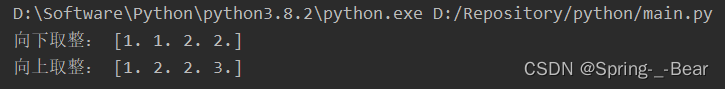
1.4.3 取整函数

程序源码：

import numpy as np

arr = np.array([1.0, 1.5, 2.0, 2.55])
print('向下取整：', np.floor(arr))
print('向上取整：', np.ceil(arr))

运行示例：

在这里插入图片描述

1.4.4 算数运算

程序源码：

import numpy as np

arr1 = np.array([1, 2, 3, 4])
arr2 = np.array([4, 3, 2, 1])

print('加：', np.add(arr1, arr2))
print('减：', np.subtract(arr1, arr2))
print('乘：', np.multiply(arr1, arr2))
print('除：', np.divide(arr1, arr2))
print('取余：', np.mod(arr1, arr2))
print('乘方：', np.power(arr1, arr2))

运行示例：

在这里插入图片描述

1.4.5 统计函数

程序源码：

import numpy as np

arr = np.arange(6).reshape(2, 3)
print('维度最小值：', np.amin(arr, 1))
print('维度最大值：', np.amax(arr, 0))
print('中位数：', np.median(arr))
print('平均数：', np.mean(arr))

运行示例：

在这里插入图片描述

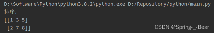
1.4.6 排序函数

程序源码：

import numpy as np

arr = np.array([[3, 5, 1], [2, 8, 7]])
print('排序：')
print(np.sort(arr, axis=1))

运行示例：

在这里插入图片描述

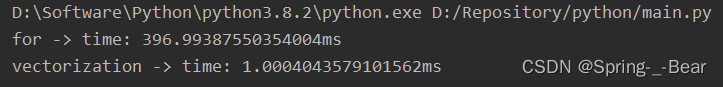
1.5 向量化编程

在某些情况下，在 Python 中使用 for 循环效率很低，此时可以选用向量化编程。

程序源码：

import numpy as np
import time

arr1 = np.random.rand(1000000)
arr2 = np.random.rand(1000000)

# 使用 for 循环
result = 0
start = time.time()
for i in range(1000000):
    result += arr1[i] * arr2[i]
end = time.time()
duration = str(1000 * (end - start)) + 'ms'
print('for -> time: %s' % duration)

# 使用向量化
start = time.time()
result = np.dot(arr1, arr2)
end = time.time()
duration = str(1000 * (end - start)) + 'ms'
print('vectorization -> time: %s' % duration)

运行示例：

在这里插入图片描述

第 2 章 Pandas

pandas 是基于 NumPy 的一种工具，该工具是为解决数据分析任务而创建的。Pandas 纳入了大量库和一些标准的数据模型，提供了高效地操作大型数据集所需的工具。pandas 提供了大量能使我们快速便捷地处理数据的函数和方法。你很快就会发现，它是使 Python 成为强大而高效的数据分析环境的重要因素之一。

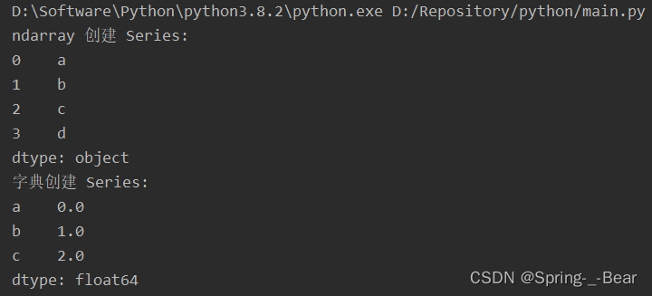
2.1 Series

pandas.Series(data=None, index=None, dtype=None, name=None, copy=False, fastpath=False)

程序源码：

import pandas as pd
import numpy as np

# pandas.Series(data=None, index=None, dtype=None, name=None, copy=False, fastpath=False)
print('ndarray 创建 Series:')
print(pd.Series(np.array(['a', 'b', 'c', 'd'])))
print('字典创建 Series:')
print(pd.Series({'a': 0., 'b': 1., 'c': 2.}))

运行示例：

在这里插入图片描述

2.2 DataFrame

DataFrame 既有行索引，也有列索引，可以看作是 Series 组成的字典，每个 Series 看作 DataFrame 的一列。

2.2.1 创建 DataFrame

程序源码：

import pandas as pd
import numpy as np

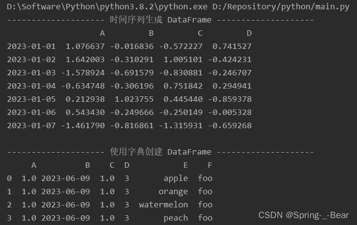
print('-------------------- 时间序列生成 DataFrame --------------------')
# 生成作为行索引的时间序列
row_dates = pd.date_range('20230101', periods=7)
# 使用随机生成的 numpy 数组作为数据，传入列索引 ABCD
df = pd.DataFrame(np.random.randn(7, 4), index=row_dates, columns=list('ABCD'))
print(df)

print('\n-------------------- 使用字典创建 DataFrame --------------------')
df = pd.DataFrame({
    'A': 1.,
    'B': pd.Timestamp('20230609'),
    'C': pd.Series(1, index=list(range(4)), dtype='float32'),
    'D': np.array([3] * 4, dtype='int32'),
    'E': pd.Categorical(['apple', 'orange', 'watermelon', 'peach']),
    'F': 'foo'
})
print(df)

运行示例：

在这里插入图片描述

2.2.2 查看 DataFrame 中的数据

程序源码：

import pandas as pd
import numpy as np

df = pd.DataFrame(
    data=np.arange(30).reshape(6, 5),
    index=['a', 'b', 'c', 'd', 'e', 'f'],
    columns=['A', 'B', 'C', 'D', 'E']
)

print('前 2 条数据：')
print(df.head(2))
print('尾 2 条数据：')
print(df.tail(2))

print('\n行索引：', df.index)
print('列索引：', df.columns)
print('数据值：')
print(df.values)

print('\n根据列名切片：')
print(df.loc['a':'f':2, 'A'])

print('\n数据详细信息：')
print(df.describe())

运行示例：

在这里插入图片描述

2.2.3 DataFrame 数据的操作

程序源码：

import pandas as pd
import numpy as np

df = pd.DataFrame(
    data=np.arange(30).reshape(6, 5),
    index=['a', 'b', 'c', 'd', 'e', 'f'],
    columns=['A', 'B', 'C', 'D', 'E']
)

print('删除指定的行：')
df1 = df.drop(['a'], axis=0)
print(df1)
print('删除指定的列：')
df2 = df.drop(['A'], axis=1)
print(df2)

print('\n合并 DataFrame：')
print(pd.concat([df1, df2]))

print('\n还原索引：')
# 使用 reset_index 方法还原索引，让原索引变为数据中的一列
df.reset_index(inplace=True)
print(df)

运行示例：

在这里插入图片描述

2.2.4 DataFrame 获取数据

程序源码：

import pandas as pd

df = pd.DataFrame({'A': [1, 2, 3], 'B': [4, 5, 6]})
for column_name, column_data in df.items():
    print("列名：", column_name)
    print("列数据：")
    print(column_data)
    print()

运行示例：

在这里插入图片描述

2.2.5 Pandas 统计函数

程序源码：

import pandas as pd
import numpy as np

print('Series 逐元素变化百分比：')
print(pd.Series([1, 2, 3, 4, 5, 4]).pct_change())
print('DataFrame 逐元素变化百分比：')
print(pd.DataFrame(np.random.randn(5, 2)).pct_change())

s1 = pd.Series(np.random.randn(10))
s2 = pd.Series(np.random.randn(10))
print('\nSeries 计算协方差：', s1.cov(s2))
df = pd.DataFrame(np.random.randn(10, 5), columns=['a', 'b', 'c', 'd', 'e'])
print('DataFrame 列之间协方差：', df['a'].cov(df['b']))

print('\nDataFrame 数据排名：')
print(df.rank())

运行示例：

在这里插入图片描述

2.2.6 Pandas 中缺失数据的简单操作

程序源码：

import pandas as pd
import numpy as np

df = pd.DataFrame(
    data=np.random.randn(5, 3),
    index=['a', 'c', 'e', 'f', 'h'],
    columns=['one', 'two', 'three']
)

print('设置新索引：')
df1 = df.reindex(['a', 'b', 'c', 'd', 'e', 'f', 'g', 'h'])
print(df1)

print('\n检查列数据是否缺失：', df1['one'].isnull())

# 列数据不全为 NaN 时 NaN 被视作 0 参与运算
print('\n缺失列数据求和：', df1['one'].sum())

print('\n标量值填充 NaN:')
print(df1.fillna(0))

print('\n删除 NaN:')
print(df1.dropna())

运行示例：

在这里插入图片描述

第 3 章 Matplotlib

Matplotlib 是一个用于绘制图表和可视化数据的 Python 库。它是一个强大而灵活的工具，被广泛用于数据分析、科学计算、工程应用和可视化任务中。

Matplotlib 提供了一种类似于 MATLAB 的绘图接口，使用户能够轻松创建各种类型的图表，包括线图、散点图、柱状图、饼图、3D 图形等。它支持各种各样的图形定制选项，可以对图形进行完全控制，包括标签、标题、颜色、线型、线宽等。

3.1 正弦函数图

程序源码：

import numpy as np
import matplotlib.pyplot as plt

# [darkgrid]暗网格 [whitegrid]白网格 [dark]全黑 [white]全白 全刻度（默认）
plt.style.use('seaborn-v0_8-darkgrid')
x = np.arange(0, 3 * np.pi, 0.1)
y = np.sin(x)
plt.plot(x, y)
plt.show()

运行示例：

在这里插入图片描述

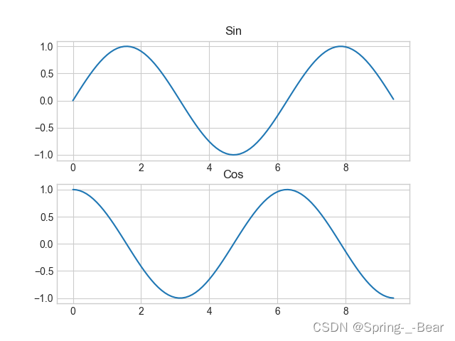
3.2 子图

程序源码：

import numpy as np
import matplotlib.pyplot as plt

plt.style.use('seaborn-v0_8-whitegrid')
x = np.arange(0, 3 * np.pi, 0.1)
sin_x = np.sin(x)
cos_x = np.cos(x)
# 第一个子图
plt.subplot(2, 1, 1)
plt.plot(x, sin_x)
plt.title('Sin')
# 第二个子图
plt.subplot(2, 1, 2)
plt.plot(x, cos_x)
plt.title('Cos')

plt.show()

运行示例：

在这里插入图片描述

3.3 图形参数

程序源码：

import numpy as np
import matplotlib.pyplot as plt

plt.style.use('seaborn-v0_8-dark')
# 创建一个 8*6 大小的画布，dpi=80 表示分辨率每英尺 80 点
plt.figure(figsize=(8, 6), dpi=80)
plt.subplot(1, 1, 1)
# numpy 准备数据
x = np.linspace(-np.pi, np.pi, 256, endpoint=True)
sin_x, cos_x = np.sin(x), np.cos(x),
# 绘制一个蓝色的，线宽为 1 个像素的余弦曲线，图例标签 Blue，linestyle 表示曲线的样式
plt.plot(x, cos_x, color='blue', linewidth=1.0, label='Blue', linestyle='--')
plt.plot(x, sin_x, color='green', linewidth=1.0, label='Green', linestyle='-.')
# 显式设置的图例
plt.legend()
# 设置 X 轴范围和刻度
plt.xlim(-4.0, 4.0)
plt.xticks(np.linspace(-4, 4, 9, endpoint=True))
plt.ylim(-1.0, 1.0)
plt.yticks(np.linspace(-1, 1, 5, endpoint=True))

# 保存图像
plt.savefig('3.3.png', dpi=72)
plt.show()

运行示例：

在这里插入图片描述

3.4 散点图

程序源码：

import numpy as np
import matplotlib.pyplot as plt

x = np.random.randint(0, 20, 15)
y = np.random.randint(0, 20, 15)
# 绘制散点图
plt.scatter(x, y)
plt.savefig('3.4.png')
plt.show()

运行示例：

在这里插入图片描述

3.5 柱状图

程序源码：

import matplotlib.pyplot as plt
from pylab import mpl

# 解决中文不显示的问题
mpl.rcParams['font.sans-serif'] = ['SimHei']

level = ['优秀', '不错', '一般']
x = range(len(level))
y = [1, 3, 2]

plt.figure(dpi=100)
# 绘制柱状图
plt.bar(x, y, width=0.5, color=['b', 'r', 'g'])
# 修改 X 轴的刻度显示
plt.xticks(x, level)
# 添加网格显示
plt.grid(linestyle='--', alpha=0.5)

plt.savefig('3.5.png')
plt.show()

运行示例：

在这里插入图片描述

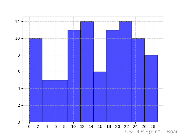
3.6 直方图

程序源码：

import matplotlib.pyplot as plt
import numpy as np

arr = np.random.randint(0, 30, 90)
plt.figure(dpi=100)
# 计算组数
group_num = int((max(arr) - min(arr)) / 2)
# 绘制直方图
plt.hist(arr, facecolor='blue', edgecolor='black', alpha=0.7)
# 修改 X 轴刻度显示
plt.xticks(range(min(arr), max(arr))[::2])
# 添加网格显示
plt.grid(linestyle='--', alpha=0.5)

plt.savefig('3.6.png')
plt.show()

运行示例：

在这里插入图片描述

第 4 章 Scipy

Scipy（Scientific Python）是一个开源的 Python 科学计算库，用于解决科学和工程中的各种数值计算问题。它建立在 NumPy（Numerical Python）库之上，并与其他科学计算库如 Matplotlib、pandas 等进行协作。

Scipy 提供了许多常用的数值算法和工具，包括数值积分、优化、线性代数、插值、信号和图像处理、稀疏矩阵等。它的目标是提供高效、易用和可扩展的数值计算功能，以支持科学计算和数据分析。

4.1 常量

程序源码：

from scipy.constants import *

print('scipy.PI:', pi)
print('真空光速：', speed_of_light)
print('普朗克常量：', h)
print('牛顿引力常数：', G)
print('电子质量：', electron_mass)

运行示例：

在这里插入图片描述

4.2 傅里叶变换

程序源码：

import numpy as np
from scipy.fftpack import fft, ifft, dct, idct

arr = np.array([1.0, 2.0, 1.0, -1.0, 1.5])

print('快速傅里叶变换：')
y = fft(arr)
print(y)
print('快速傅里叶逆变换：')
print(ifft(y))
print('离散余弦变换：')
y = dct(arr)
print(y)
print('离散余弦逆变换：')
print(idct(y))

运行示例：

在这里插入图片描述

4.3 插值

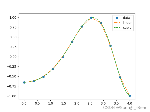
4.3.1 拟合函数

程序源码：

import numpy as np
from scipy import interpolate as ip
import matplotlib.pyplot as plt

x = np.linspace(0, 4, 12)
y = np.cos(x ** 2 / 3 + 4)

# interp1d 根据输入的点，创建拟合函数
f1 = ip.interp1d(x, y, kind='linear')
f2 = ip.interp1d(x, y, kind='cubic')
x_new = np.linspace(0, 4, 30)
plt.plot(x, y, 'o', x_new, f1(x_new), '-.', x_new, f2(x_new), '--')
plt.legend(['data', 'linear', 'cubic', 'nearest'])

plt.savefig('4.3.png')
plt.show()

运行示例：

在这里插入图片描述

4.3.2 噪声插值

程序源码：

import numpy as np
import matplotlib.pyplot as plt
from scipy.interpolate import UnivariateSpline

x = np.linspace(-3, 3, 50)
# 通过 random 方法添加噪声数据
y = np.exp(-x ** 2) + 0.1 * np.random.randn(50)

# 平滑参数使用默认值
spl = UnivariateSpline(x, y)
xs = np.linspace(-3, 3, 1000)
plt.plot(xs, spl(xs), 'blue', lw=3)

# 设置平滑参数
spl.set_smoothing_factor(0.5)
plt.plot(xs, spl(xs), 'green', lw=3)

# 设置平滑参数为 0
spl.set_smoothing_factor(0)
plt.plot(xs, spl(xs), 'yellow', lw=3)

plt.savefig('4.3.2.png')
plt.show()

运行示例：

在这里插入图片描述

4.4 线性代数运算

程序源码：

import numpy as np
from scipy import linalg

arr1 = np.array([[1, 3, 5], [2, 5, 1], [2, 3, 8]])
arr2 = np.array([10, 8, 3])
print('解线性方程：', linalg.solve(arr1, arr2))

print('\n计算行列式：', linalg.det(np.array([[3, 4], [7, 8]])))

eigenvalues, eigenvectors = np.linalg.eig(arr1)
print('\n特征值：', eigenvalues)
print('特征向量：')
print(eigenvectors)

print('\n奇异值分解：')
A = np.array([[1, 2, 3], [4, 5, 6], [7, 8, 9]])
U, s, VT = np.linalg.svd(A)
print("U:\n", U)
print("s:\n", s)
print("VT:\n", VT)

运行示例：

在这里插入图片描述

第 5 章 Scikit-learn

Scikit-learn（简称 sklearn）是一个开源的机器学习库，它建立在 NumPy、SciPy 和 Matplotlib 之上，并提供了用于数据预处理、模型选择、模型评估和部署的丰富工具集。Scikit-learn 为 Python 提供了简单而高效的机器学习算法实现，使得机器学习任务更加容易上手和快速实现。

5.1 特征工程

5.1.1 特征抽取

程序源码：

from sklearn.feature_extraction import DictVectorizer

data = [
    {'name': '张三', 'age': 20},
    {'name': '李四', 'age': 24},
    {'name': '王五', 'age': 18}
]
transfer = DictVectorizer(sparse=False)
# 将数据 data 进行 One-Hot 编码，即将字典形式的数据转换为矩阵表示，其中每个特征都被展开为二进制的 One-Hot 编码
data = transfer.fit_transform(data)
'''
特征结果：是经过 One-Hot 编码后的特征矩阵。每行表示一个样本，每列代表一个特征。
在这个例子中，'name' 被展开为三个二进制特征列，分别表示 '张三'、'李四' 和 '王五'。'age' 则是一个数值特征列
'''
print('特征结果：')
print(data)
# 特征名字：是每个特征的名称。在这个例子中，'age' 是数值特征，而 'name' 则展开为 '张三'、'李四'和 '王五' 三个特征列
print('特征名字：', transfer.get_feature_names_out())

运行示例：

在这里插入图片描述

5.1.2 归一化

程序源码：

import pandas as pd
from sklearn.preprocessing import MinMaxScaler

df = pd.DataFrame([[30, 1, 5], [27, 3, 6], [34, 2, 6]], columns=['a', 'b', 'c'])
transfer = MinMaxScaler(feature_range=(0, 1))
# 归一化：异常点会影响到最终的归一化结果
data = transfer.fit_transform(df[['a', 'b', 'c']])
print(data)

运行示例：

在这里插入图片描述

5.1.3 标准化

程序源码：

import pandas as pd
from sklearn.preprocessing import StandardScaler

df = pd.DataFrame([[30, 1, 5], [27, 3, 6], [34, 2, 6]], columns=['a', 'b', 'c'])
transfer = StandardScaler()
# 标准化
data = transfer.fit_transform(df[['a', 'b', 'c']])
print(data)

运行示例：

在这里插入图片描述

5.2 回归算法

程序源码：

"""
使用线性回归预测波士顿房价
"""
from sklearn.datasets import load_boston
from sklearn.linear_model import SGDRegressor
from sklearn.model_selection import train_test_split
from sklearn.preprocessing import StandardScaler
from sklearn.metrics import mean_squared_error
import matplotlib.pyplot as plt

'''
查看数据的一些属性
'''
boston = load_boston()
print('数据维度：', boston.data.shape)
print('房价数据：', boston.data)
print('特征：', boston.feature_names)
print('标签：', boston.target)

'''
划分数据集
'''
x_train, x_test, y_train, y_test = train_test_split(boston.data, boston.target, test_size=0.2, random_state=6)
print('\n训练集：', x_train)
print('训练集维度：', x_train.shape)
print('测试集：', x_test)
print('测试集维度：', x_test.shape)

'''
数据标准化
'''
transfer = StandardScaler()
x_train = transfer.fit_transform(x_train)
x_test = transfer.transform(x_test)
# 数据在标准化后数值发生了变化，但是数据维度没有变化
print('\n标准化：', x_train)
print('标准化后的维度：', x_train.shape)

'''
线性回归算法
'''
estimator = SGDRegressor()
# 使用 fit 方法填充数据进行训练
estimator.fit(x_train, y_train)
# 预测
y_predict = estimator.predict(x_test)
print('\n预测：')
print(y_predict)

'''
均方误差
'''
error = mean_squared_error(y_test, y_predict)
print('\n均方误差：')
print(error)

'''
可视化结果查看
'''
plt.figure(figsize=(10, 8))
plt.xlabel('x', fontsize=14)
plt.ylabel('y', fontsize=14)
plt.plot([i for i in range(len(y_test))], y_test, linestyle=':', marker='o', label='true')
plt.plot([i for i in range(len(y_test))], y_predict, linestyle=':', marker='o', label='predict')
plt.legend()

plt.show()

运行示例：

在这里插入图片描述

5.3 分类算法

5.3.1 逻辑回归

程序源码：

"""
使用逻辑回归来进行癌症分类预测
"""
from sklearn.model_selection import train_test_split
from sklearn.linear_model import LogisticRegression
from sklearn.preprocessing import StandardScaler
import pandas as pd
import numpy as np

column_names = ['Sample Code Number', 'Clump Thickness', 'Uniformity of Cell Size', 'Uniformity of Cell Shape',
                'Marginal Adhesion', 'Simple Epithelial Cell Size', 'Bare Nuclei', 'Bland Chromatin',
                'Normal Nucleoli', 'Mitoses', 'Class']
data = pd.read_csv(
    r'https://archive.ics.uci.edu/ml/machine-learning-databases/breast-cancer-wisconsin/breast-cancer-wisconsin.data',
    names=column_names
)

# 删除缺失值
data = data.replace(to_replace='?', value=np.nan)
data = data.dropna()

# 取出特征值
x = data[column_names[1:10]]
y = data[column_names[10]]

# 分割数据集，测试集占比 30%
x_train, x_test, y_train, y_test = train_test_split(x, y, test_size=0.3)

# 标准化
std = StandardScaler()
x_train = std.fit_transform(x_train)
x_test = std.transform(x_test)

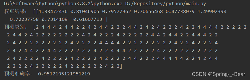
# 逻辑回归
lr = LogisticRegression()
lr.fit(x_train, y_train)

print('权重结果：', lr.coef_)
print('预测类别：', lr.predict(x_test))
print('预测准确率：', lr.score(x_test, y_test))

运行示例：

在这里插入图片描述

5.3.2 KNN

程序源码：

"""
使用 KNN 算法实现鸢尾花种类预测
"""
from sklearn.datasets import load_iris
from sklearn.model_selection import train_test_split
from sklearn.preprocessing import StandardScaler
from sklearn.neighbors import KNeighborsClassifier

iris = load_iris()
# 分割数据集
x_train, x_test, y_train, y_test = train_test_split(iris.data, iris.target, test_size=0.2, random_state=22)

# 标准化
std = StandardScaler()
x_train = std.fit_transform(x_train)
x_test = std.transform(x_test)

# 实例化 KNN 分类器
estimator = KNeighborsClassifier(n_neighbors=9)
estimator.fit(x_train, y_train)

# 模型评估
y_predict = estimator.predict(x_test)

print('预测结果：', y_predict)
print('比对真实值和预测值：', y_predict == y_test)
print('准确率：', estimator.score(x_test, y_test))

运行示例：

在这里插入图片描述

5.3.3 决策树

程序源码：

"""
使用决策树算法实现泰坦尼克号乘客生存预测
"""
from sklearn.tree import DecisionTreeClassifier
from sklearn.feature_extraction import DictVectorizer
from sklearn.model_selection import train_test_split
import pandas as pd

# get `titanic_data.csv` from `https://github.com/rashida048/Datasets/blob/master/titanic_data.csv`
file = open(r'titanic_data.csv')
titan = pd.read_csv(file)

# 取出特征值
x = titan[['Pclass', 'Age', 'Sex']].copy()
y = titan['Survived'].copy()

# 缺失值进行字典特征抽取
x['Age'].fillna(x['Age'].mean(), inplace=True)

# 将字典型数据（包含类别特征）转换为数值特征矩阵
dv = DictVectorizer(sparse=False)
x = dv.fit_transform(x.to_dict(orient='records'))
print(dv.get_feature_names_out())
print(x)

# 分割数据集
x_train, x_test, y_train, y_test = train_test_split(x, y, test_size=0.3)

# 进行决策树的建立和预测，指定树的深度大小为 5
dtc = DecisionTreeClassifier(criterion='entropy', max_depth=5)
dtc.fit(x_train, y_train)
print('预测的准确率为：', dtc.score(x_test, y_test))

运行示例：

在这里插入图片描述

5.4 聚类算法

k-means 和 DBSCAN 是两种常见的聚类算法，它们在聚类的方式和原理上有一些区别和联系。

区别：

聚类方式：k-means 是基于距离的划分聚类算法，将数据点划分为 k 个簇，每个簇以其质心（中心点）来表示；DBSCAN 是一种基于密度的聚类算法，通过寻找高密度区域来划分簇，簇可以具有不同的形状和大小。
簇的数量：k-means 需要预先指定聚类的数量 k，而 DBSCAN 可以自动确定簇的数量，不需要事先指定。
数据分布：k-means 对于具有明显凸出的簇和相对均匀分布的数据效果较好；DBSCAN 对于具有不同形状和密度的簇以及噪声点的数据具有较好的适应性。
对噪声的处理：k-means 对于噪声数据点敏感，将其分配到最近的簇；DBSCAN 能够自动识别和排除噪声点。

联系：

相同点：k-means 和 DBSCAN 都是聚类算法，用于将数据集划分为不同的簇。
数据点分类：两种算法都会为每个数据点分配一个簇标签。
距离度量：k-means 和 DBSCAN 都使用距离度量来计算数据点之间的相似性或差异性。
迭代过程：两种算法都使用迭代的方式来优化聚类结果，直到满足停止条件。

选择使用 k-means 还是 DBSCAN 取决于数据的特点和应用需求。如果你已经知道聚类的数量，并且数据分布相对均匀，可以尝试使用 k-means。如果你不确定聚类数量，数据分布复杂，或者希望自动识别和排除噪声点，可以尝试使用 DBSCAN。

5.4.1 K-means

程序源码：

"""
使用 K-means 聚类算法实现鸢尾花的聚类操作
"""
import matplotlib.pyplot as plt
from sklearn.cluster import KMeans
from sklearn import datasets

iris = datasets.load_iris()
# 抽取特征空间中的 4 个维度
x = iris.data[:, :4]
print('数据维度：', x.shape)

# 绘制数据分布图
plt.scatter(x[:, 0], x[:, 1], c='red', marker='o', label='data')
plt.xlabel('sepal length')
plt.ylabel('sepal width')
plt.legend(loc=2)
plt.show()

# 构造聚类器
estimator = KMeans(n_clusters=3)
# 聚类
estimator.fit(x)
# 获取聚类标签
label_pred = estimator.labels_

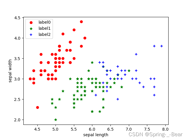
# 绘制 k-means 结果
x0 = x[label_pred == 0]
x1 = x[label_pred == 1]
x2 = x[label_pred == 2]

plt.scatter(x0[:, 0], x0[:, 1], c='red', marker='o', label='label0')
plt.scatter(x1[:, 0], x1[:, 1], c='green', marker='*', label='label1')
plt.scatter(x2[:, 0], x2[:, 1], c='blue', marker='+', label='label2')
plt.xlabel('sepal length')
plt.ylabel('sepal width')
plt.legend(loc=2)

plt.savefig('5.4.1.png')
plt.show()

运行示例：

在这里插入图片描述

5.4.2 DBSCAN

程序源码：

"""
使用 DBSCAN 聚类算法实现鸢尾花的聚类操作
"""
import matplotlib.pyplot as plt
from sklearn.cluster import DBSCAN
from sklearn import datasets

iris = datasets.load_iris()
# 抽取特征空间中的 4 个维度
x = iris.data[:, :4]
print('数据维度：', x.shape)

# 绘制数据分布图
plt.scatter(x[:, 0], x[:, 1], c='red', marker='o', label='data')
plt.xlabel('sepal length')
plt.ylabel('sepal width')
plt.legend(loc=2)
plt.show()

# 构造聚类器
estimator = DBSCAN(eps=0.4, min_samples=4)

# 聚类
estimator.fit(x)
# 获取聚类标签
label_pred = estimator.labels_

# 绘制 DBSCAN 结果
x0 = x[label_pred == 0]
x1 = x[label_pred == 1]
x2 = x[label_pred == 2]

plt.scatter(x0[:, 0], x0[:, 1], c='red', marker='o', label='label0')
plt.scatter(x1[:, 0], x1[:, 1], c='green', marker='*', label='label1')
plt.scatter(x2[:, 0], x2[:, 1], c='blue', marker='+', label='label2')
plt.xlabel('sepal length')
plt.ylabel('sepal width')
plt.legend(loc=2)

plt.savefig('5.4.2.png')
plt.show()

运行示例：

在这里插入图片描述

第 6 章常用标准库

6.1 sys 模块

程序源码：

import sys

print('当前系统平台：', sys.platform)
print('Python 版本：', sys.version)
print('模块搜索路径：')
for path in sys.path:
    print(path)
print('系统退出：-1')
sys.exit(-1)

运行示例：

在这里插入图片描述

6.2 os 模块

6.2.1 基础使用

程序源码：

import os

print('当前进程 ID：', os.getpid())
print('父进程 ID：', os.getppid())
print('当前工程路径：', os.getcwd())
os.chdir('c:\\')
print('修改当前路径：', os.getcwd())
print('列举目录：', os.listdir('D:\\Repository'))
print('输出指定目录下所有文件：')
for root, dirs, files in os.walk('D:\\Repository\\python', topdown=False):
    for name in files:
        print(os.path.join(root, name))
    for name in dirs:
        print(os.path.join(root, name))

运行示例：

在这里插入图片描述

6.2.2 路径操作

程序源码：

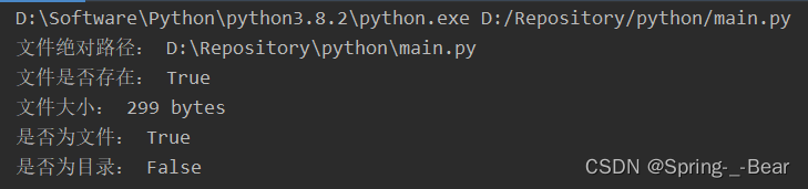
import os

print('文件绝对路径：', os.path.abspath('main.py'))
print('文件是否存在：', os.path.exists('main.py'))
print('文件大小：', os.path.getsize('main.py'), 'bytes')
print('是否为文件：', os.path.isfile('main.py'))
print('是否为目录：', os.path.isdir('main.py'))

运行示例：

在这里插入图片描述

6.3 time 模块

程序源码：

import time

time_now = time.time()
print('时间戳：', time_now)
time_tuple = time.localtime(time_now)
print('时间元组：', time_tuple)
print('本地时间：', time.asctime(time_tuple))
print('时间格式化：', time.strftime('%Y-%m-%d %H:%M:%S', time_tuple))

运行示例：

在这里插入图片描述

第 7 章常用数据结构

7.1 单链表

程序源码：

class LinkedListNode:
    def __init__(self, data):
        self.data = data
        self.next = None


class LinkedList:
    # 初始化链表，设置链表头为空
    def __init__(self):
        self._head = None

    # 判断表头是否为空值
    def is_empty(self):
        return self._head is None

    # 计算链表节点长度
    def length(self):
        node = self._head
        count = 0
        while node:
            count += 1
            node = node.next
        return count

    # 在表头添加数据
    def add(self, data):
        new_node = LinkedListNode(data)
        # 将新节点插入到表头前
        new_node.next = self._head
        # 将新插入的节点设为头节点
        self._head = new_node

    # 打印链表
    def print_list(self):
        if self._head:
            cur = self._head
            while cur:
                print(cur.data, end=' ')
                cur = cur.next

    # 链表尾添加节点
    def append(self, data):
        new_node = LinkedListNode(data)
        if self._head is None:
            self._head = new_node
        else:
            pre, cur = None, self._head
            while cur:
                pre, cur = cur, cur.next
            # 将新节点连接到链表尾部
            pre.next = new_node

    # 在指定索引位置插入节点
    def insert(self, data, index):
        # 头插
        if index <= 0:
            self.add(data)
        # 尾插
        elif index >= self.length():
            self.append(data)
        else:
            new_node = LinkedListNode(data)
            pre, cur = self._head, self._head.next
            count = 1
            while cur:
                if count == index:
                    # 将新节点插入到 pre 和 cur 之间 pre -> new_node -> next
                    pre.next, new_node.next = new_node, cur
                    break

                pre, cur = cur, cur.next
                count += 1

    # 根据元素值移除元素
    def remove(self, data):
        if self.is_empty():
            raise Exception("Can't remove the element because linked list is empty.")

        pre, cur = None, self._head
        while cur:
            if cur.data == data:
                if pre is None:
                    # 删除表头节点
                    self._head = cur.next
                else:
                    # 删除目标节点
                    pre.next = cur.next
                return cur.data
            pre, cur = cur, cur.next

        raise Exception("Can't remove the element because it not exists in the linked list.")

    # 搜索元素，搜索成功返回下标
    def search(self, data):
        if self.is_empty():
            return -1
        else:
            cur = self._head
            index = 0
            while cur:
                if cur.data == data:
                    # 找到了数据，返回其在单链表中的索引号
                    return index
                index += 1
                cur = cur.next
            return -1


if __name__ == '__main__':
    linked_list = LinkedList()
    linked_list.add(1)
    linked_list.append(2)
    linked_list.append(3)
    linked_list.append(4)
    linked_list.append(5)

    print('链表是否为空：', str(linked_list.is_empty()))
    print('链表节点个数：', str(linked_list.length()))
    print('遍历链表：', end='', )
    linked_list.print_list()

    linked_list.insert(6, 2)
    print('\n搜索元素：', linked_list.search(6))
    print('移除元素：', linked_list.remove(6))

运行示例：

在这里插入图片描述

7.2 双链表

程序源码：

class DoubleLinkedListNode:
    def __init__(self, data):
        self.data = data
        self.next = None
        self.prev = None


class DoubleLinkedList:
    def __init__(self):
        self._head = None

    # 链表是否为空
    def is_empty(self):
        return self._head is None

    # 返回链表长度
    def length(self):
        cur = self._head
        count = 0
        while cur:
            count += 1
            cur = cur.next
        return count

    # 打印双链表
    def print_list(self):
        cur = self._head
        while cur:
            print(cur.data, end=' ')
            cur = cur.next

    # 元素头插
    def add(self, data):
        node = DoubleLinkedListNode(data)

        if self.is_empty():
            self._head = node
        else:
            # 新节点后继指向头节点
            node.next = self._head
            # 头节点前驱指向新节点
            self._head.prev = node
            # 新节点设置为头节点
            self._head = node

    # 元素尾插
    def append(self, data):
        node = DoubleLinkedListNode(data)

        if self.is_empty():
            self._head = node
        else:
            cur = self._head
            # 移动到尾节点的上一节点
            while cur.next is not None:
                cur = cur.next
            # 尾节点后续指向新节点
            cur.next = node
            # 新节点前驱节点指向为节点
            node.prev = cur

    # 查找元素
    def is_exists(self, data):
        cur = self._head

        while cur is not None:
            if cur.data == data:
                return True
            cur = cur.next

        return False

    # 在指定下标位置插入元素
    def insert(self, data, index):
        if index <= 0:
            self.add(data)
        elif index > self.length() - 1:
            self.append(data)
        else:
            node = DoubleLinkedListNode(data)
            cur = self._head
            count = 0

            # 移动到目标位置的前一个位置
            while count < index - 1:
                count += 1
                cur = cur.next

            # 将新元素插入到指定下标位置
            node.prev = cur
            node.next = cur.next
            cur.next.prev = node
            cur.next = node

    # 删除元素
    def remove(self, data):
        if self.is_empty():
            return -1
        else:
            cur = self._head

            # 删除头节点
            if cur.data == data:
                # 只有头节点
                if cur.next is None:
                    self._head = None
                else:
                    # 头节点的下一节点前驱指向空
                    cur.next.prev = None
                    # 下一节点设为头节点
                    self._head = cur.next.prev
                return

            while cur is not None:
                if cur.data == data:
                    # 移除目标节点
                    cur.prev.next = cur.next
                    cur.next.prev = cur.prev
                    return cur.data
                cur = cur.next


if __name__ == '__main__':
    double_linked_list = DoubleLinkedList()
    double_linked_list.add(1)
    double_linked_list.append(2)
    double_linked_list.append(3)
    double_linked_list.append(4)
    double_linked_list.append(5)

    print('链表是否为空：', double_linked_list.is_empty())
    print('链表节点个数：', double_linked_list.length())
    print('遍历链表：', end='')
    double_linked_list.print_list()

    double_linked_list.insert(6, 2)
    print('\n搜索元素：', double_linked_list.is_exists(6))
    print('移除元素：', double_linked_list.remove(6))

运行示例：

在这里插入图片描述

7.3 二叉树

程序源码：

class BinaryTreeNode:
    def __init__(self):
        self.data = '#'
        self.left = None
        self.right = None


# 打印节点数据
def print_node(root_node):
    if root_node.data != '#':
        print(root_node.data, end='->')


class BinaryTree:
    def create(self, root):
        data = input('===>')
        if data == '#':
            root = None
        else:
            root.data = data

            root.left = BinaryTreeNode()
            self.create(root.left)
            root.right = BinaryTreeNode()
            self.create(root.right)

    # 先序遍历
    def pre_order(self, root):
        if root is not None:
            print_node(root)
            self.pre_order(root.left)
            self.pre_order(root.right)

    # 中序遍历
    def in_order(self, root):
        if root is not None:
            self.in_order(root.left)
            print_node(root)
            self.in_order(root.right)

    # 后续遍历
    def post_order(self, root):
        if root is not None:
            self.post_order(root.left)
            self.post_order(root.right)
            print_node(root)


if __name__ == '__main__':
    node = BinaryTreeNode()
    tree = BinaryTree()

    tree.create(node)
    print('先序遍历结果：')
    tree.pre_order(node)
    print('\n中序遍历结果：')
    tree.in_order(node)
    print('\n后序遍历结果：')
    tree.post_order(node)

运行示例：

在这里插入图片描述

附录

库名	版本
numpy	1.24.3
pandas	2.0.2
matplotlib	3.7.1
scipy	1.10.1
scikit-learn	1.10.3

春天熊

关注

1
点赞
踩
3

收藏

觉得还不错? 一键收藏
打赏
0
评论
[Python语言程序设计]Python 课程实验

Python 由荷兰数学和计算机科学研究学会的吉多·范罗苏姆于 1990 年代初设计，作为一门叫做 ABC 语言的替代品。Python 提供了高效的高级数据结构，还能简单有效地面向对象编程。Python 语法和动态类型，以及解释型语言的本质，使它成为多数平台上写脚本和快速开发应用的编程语言，随着版本的不断更新和语言新功能的添加，逐渐被用于独立的、大型项目的开发。
复制链接

扫一扫