


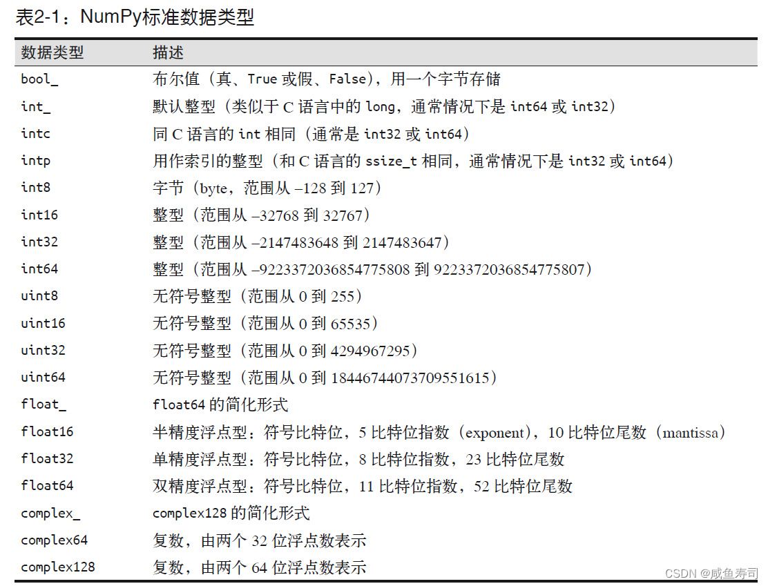
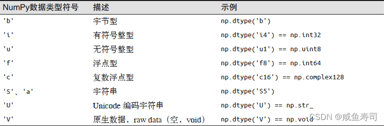
数据类型
从头创建Numpy矩阵
import numpy as np
a = np.zeros((3,3), dtype=int)
b = np.ones((4,4))
# 用第二个参数填充矩阵
c = np.full((5,5), 114)
d = np.arange(5,14,2)
# 一维矩阵,从1到14共划分5个点
e = np.linspace(1,14,5)
f = np.random.random((1,9))
# 高斯分布,均值为1,方差为9
g = np.random.normal(1,9,(8,10))
# 整数矩阵,元素为8-10
h = np.random.randint(8,10,(5,14))
# 对角矩阵
i = np.eye(4)
j = np.empty((5,5))
print(a,'\n')
print(b,'\n')
print(c,'\n')
print(d,'\n')
print(e,'\n')
print(f,'\n')
print(g,'\n')
print(h,'\n')
print(i,'\n')
print(j)
输出结果:
runcell('[1]', 'D:/Download/Numpy_test.py')
[[0 0 0]
[0 0 0]
[0 0 0]][[1. 1. 1. 1.]
[1. 1. 1. 1.]
[1. 1. 1. 1.]
[1. 1. 1. 1.]][[114 114 114 114 114]
[114 114 114 114 114]
[114 114 114 114 114]
[114 114 114 114 114]
[114 114 114 114 114]][ 5 7 9 11 13]
[ 1. 4.25 7.5 10.75 14. ]
[[0.99754788 0.38404322 0.89769878 0.64001409 0.79864365 0.00587426
0.24060298 0.02571805 0.86974474]][[ -2.42883103 6.55958076 -1.08847698 7.86765631 15.3364416
5.43309595 -10.10755128 -3.97506294 0.44066907 12.03037985]
[ 2.92938976 15.02462572 -9.65963732 4.2563517 -3.29301815
-1.85601016 0.63432327 0.03077856 12.83798304 -5.36509117]
[ 9.34828876 4.6916838 1.12534694 -16.23384907 -10.88859662
11.94436137 -4.42950259 -2.99541989 -15.88960588 3.90555322]
[ 0.19158792 -8.31119427 4.54304223 15.09235549 25.88781742
-0.59878842 -1.72860137 7.729361 27.94515944 -5.42564422]
[ 2.37526154 1.30766984 -4.0169404 0.86828363 -5.44062589
5.20853733 8.1877904 6.23111479 7.33052294 -5.29591986]
[ 9.04855168 -7.61928819 9.66387067 12.48155684 1.36824221
-10.15502133 2.20568686 -4.76172936 -11.86549394 -3.67921843]
[ -6.81807438 3.16669276 -2.44106965 6.88086055 -0.34887463
8.25984449 -6.02556218 -11.60013348 7.3875109 7.85789654]
[-12.81114941 1.45862671 -7.90770309 -11.56738065 7.47641083
-10.82952007 -7.18628427 6.6185245 11.02849474 3.00631948]][[8 9 8 9 9 9 8 9 8 9 8 8 8 8]
[9 8 9 9 8 8 9 8 8 8 8 9 8 9]
[8 8 9 9 8 9 8 9 8 8 8 9 8 8]
[9 8 8 9 9 8 9 8 9 9 9 8 8 9]
[9 9 8 9 8 9 8 9 8 9 8 9 9 9]][[1. 0. 0. 0.]
[0. 1. 0. 0.]
[0. 0. 1. 0.]
[0. 0. 0. 1.]][[6.23042070e-307 4.67296746e-307 1.69121096e-306 1.22383391e-307
8.34441742e-308]
[8.90104239e-307 1.33511290e-306 1.29060531e-306 1.11258854e-306
1.11261502e-306]
[1.42410839e-306 7.56597770e-307 6.23059726e-307 8.90111708e-307
1.86918699e-306]
[1.69120281e-306 1.78022206e-306 7.56599807e-307 1.11260348e-306
2.22522868e-306]
[1.37962049e-306 9.34601642e-307 1.60219035e-306 2.22522596e-306
3.91786943e-317]]
标准数据类型
第二个参数dtype可以指定矩阵标准数据类型
Numpy数组基础
数组属性
np.random.seed可以指定随机数种子,使每次随机的结果相同
np数组常用属性:
- ndim:维度
- shape:尺寸
- size:元素个数
- dtype:元素数据类型
- itemsize:元素字节数
- nbytes:数组字节数
import numpy as np
np.random.seed(41)
test = np.random.randint(1, 5, (3,3))
print(test)
print("数组维度:", test.ndim)
print("数组尺寸:", test.shape)
print("数组元素个数:", test.size)
print("数组元素数据类型:", test.dtype)
print("数组元素所用字节数:", test.itemsize)
print("整个数组所用字节数:", test.nbytes)
输出结果:
[[1 4 1]
[3 1 2]
[4 2 4]]
数组维度: 2
数组尺寸: (3, 3)
数组元素个数: 9
数组元素数据类型: int32
数组元素所用字节数: 4
整个数组所用字节数: 36
非副本视图
直接赋值传递的是类似指针的非副本视图,因此对新矩阵的修改会影响到旧矩阵,使用copy方法可以获得非视图副本
import numpy as np
test = np.random.randint(1, 3, (5,5))
test1 = test[:3, :3]
print("test:\n", test)
print("test1:\n", test1)
test1[0, 0] = 0
print("new test1:\n", test1)
print("new test:\n", test)
test2 = test.copy()
test2[0, 0] = 114514
print("test2:\n", test2)
print("test:\n", test)
test:
[[1 1 1 2 1]
[2 1 2 2 2]
[2 2 1 1 1]
[1 1 2 1 1]
[2 2 1 2 2]]
test1:
[[1 1 1]
[2 1 2]
[2 2 1]]
new test1:
[[0 1 1]
[2 1 2]
[2 2 1]]
new test:
[[0 1 1 2 1]
[2 1 2 2 2]
[2 2 1 1 1]
[1 1 2 1 1]
[2 2 1 2 2]]
test2:
[[114514 1 1 2 1]
[ 2 1 2 2 2]
[ 2 2 1 1 1]
[ 1 1 2 1 1]
[ 2 2 1 2 2]]
test:
[[0 1 1 2 1]
[2 1 2 2 2]
[2 2 1 1 1]
[1 1 2 1 1]
[2 2 1 2 2]]
数组的变形
reshape改变当前数组的shape,前后数组的size不同
newaxis改变当前数组的ndim
import numpy as np
test = np.ones((1,6))
print("test:", test)
print("shape:", test.shape)
test = test.reshape((3, 2))
print("reshape_test:\n", test)
print("shape:", test.shape)
# 通过newaxis增加维度
test = test[:, :, np.newaxis]
print("ndim_test:", test.ndim)
test: [[1. 1. 1. 1. 1. 1.]]
shape: (1, 6)
reshape_test:
[[1. 1.]
[1. 1.]
[1. 1.]]
shape: (3, 2)
ndim_test: 3
拼接和分裂
拼接
np.concatenate,第一个参数为列表,元素为拼接数组,第二个参数axis为维度
np.vstack,行拼接,列表中前一个数组拼接后在前
np.hstack,列拼接
np.dstack,第三维度拼接
import numpy as np
np.random.seed(114514)
test = np.random.randint(0, 1, (6,6))
test1 = np.array([1, 1, 4, 5, 1, 4])
test2 = test1[np.newaxis, :]
test3 = test1[:, np.newaxis]
out1 = np.concatenate([test, test2])
out2 = np.concatenate([test, test3], axis=1)
print("out1:\n", out1)
print("out2:\n", out2)
out3 = np.vstack([test, test2])
out4 = np.hstack([test, test3])
print("out3:\n", out3)
print("out4:\n", out4)
out1:
[[0 0 0 0 0 0]
[0 0 0 0 0 0]
[0 0 0 0 0 0]
[0 0 0 0 0 0]
[0 0 0 0 0 0]
[0 0 0 0 0 0]
[1 1 4 5 1 4]]
out2:
[[0 0 0 0 0 0 1]
[0 0 0 0 0 0 1]
[0 0 0 0 0 0 4]
[0 0 0 0 0 0 5]
[0 0 0 0 0 0 1]
[0 0 0 0 0 0 4]]
out3:
[[0 0 0 0 0 0]
[0 0 0 0 0 0]
[0 0 0 0 0 0]
[0 0 0 0 0 0]
[0 0 0 0 0 0]
[0 0 0 0 0 0]
[1 1 4 5 1 4]]
out4:
[[0 0 0 0 0 0 1]
[0 0 0 0 0 0 1]
[0 0 0 0 0 0 4]
[0 0 0 0 0 0 5]
[0 0 0 0 0 0 1]
[0 0 0 0 0 0 4]]
分裂
np.split,第一个参数为数组,第二个参数为元组的分裂点位置
np.vsplit,行分裂,第二个参数为列表的分裂点位置,不是从0开始
np.hsplit,列分裂,同上
np.dsplit,第三维度分裂
import numpy as np
np.random.seed(114514)
test = np.random.randint(0, 1, (6,6))
test1 = np.array([1, 1, 4, 5, 1, 4])
test2 = test1[np.newaxis, :]
test3 = test1[:, np.newaxis]
out1 = np.concatenate([test, test2])
out2 = np.concatenate([test, test3], axis=1)
print("out1:\n", out1)
print("out2:\n", out2)
out3 = np.vstack([test, test2])
out4 = np.hstack([test, test3])
print("out3:\n", out3)
print("out4:\n", out4)

s1, s2 = np.split(out1, [6], axis=0)    # 相当于np.vspilt
print("s1:\n", s1)
print("s2:\n", s2)
s3, s4 = np.hsplit(out2, [6])
print("s3:\n", s3)
print("s4:\n", s4)
out1:
[[0 0 0 0 0 0]
[0 0 0 0 0 0]
[0 0 0 0 0 0]
[0 0 0 0 0 0]
[0 0 0 0 0 0]
[0 0 0 0 0 0]
[1 1 4 5 1 4]]
out2:
[[0 0 0 0 0 0 1]
[0 0 0 0 0 0 1]
[0 0 0 0 0 0 4]
[0 0 0 0 0 0 5]
[0 0 0 0 0 0 1]
[0 0 0 0 0 0 4]]
out3:
[[0 0 0 0 0 0]
[0 0 0 0 0 0]
[0 0 0 0 0 0]
[0 0 0 0 0 0]
[0 0 0 0 0 0]
[0 0 0 0 0 0]
[1 1 4 5 1 4]]
out4:
[[0 0 0 0 0 0 1]
[0 0 0 0 0 0 1]
[0 0 0 0 0 0 4]
[0 0 0 0 0 0 5]
[0 0 0 0 0 0 1]
[0 0 0 0 0 0 4]]
s1:
[[0 0 0 0 0 0]
[0 0 0 0 0 0]
[0 0 0 0 0 0]
[0 0 0 0 0 0]
[0 0 0 0 0 0]
[0 0 0 0 0 0]]
s2:
[[1 1 4 5 1 4]]
s3:
[[0 0 0 0 0 0]
[0 0 0 0 0 0]
[0 0 0 0 0 0]
[0 0 0 0 0 0]
[0 0 0 0 0 0]
[0 0 0 0 0 0]]
s4:
[[1]
[1]
[4]
[5]
[1]
[4]]
通用函数
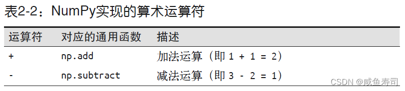
可以使用+,-,*,/,//,%,**直接运算矩阵所有元素以代替使用循环
绝对值:np.abs(),将数组的元素全部替换为绝对值
三角函数:np.sin(),np.cos(),搭配np.lincespace()和np.pi风味更佳
指数:除了**,可以使用np.exp(),np.exp2(),np.power(a, b),其中a为底数,b为指数
对数:np.log(),np.log2(),np.log10()
特殊:np.expm1()(等价于exp()-1),np.logp1()(等价于log(x+1)),np.logaddexp(a,b)(等价于log(exp(a)+exp(b))
指定输出
使用out指定输出到空向量
import numpy as np
a = np.array([1, 1, 4, 5, 1, 4])
b = np.empty(6)
np.multiply(2, a, out=b[::-1])
print(b)
[ 8. 2. 10. 8. 2. 2.]
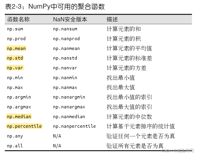
聚合
add通用函数调用reduce会返回数组的和
multiply通用函数调用reduce会返回数组的乘积
储存每次计算的结果可以使用accumulate,返回数组
外积
outer可以返回两个不同输入函数组所有元素对的通用函数运算结果矩阵
import numpy as np
a = np.array([1, 1, 4, 5, 1, 4])
b = np.multiply.outer(a, a)
print(b)
[[ 1 1 4 5 1 4]
[ 1 1 4 5 1 4]
[ 4 4 16 20 4 16]
[ 5 5 20 25 5 20]
[ 1 1 4 5 1 4]
[ 4 4 16 20 4 16]]
聚合
import numpy as np
import matplotlib.pyplot as plt
import seaborn
seaborn.set()
plt.rcParams['font.sans-serif'] = ['SimHei']  # 用来正常显示中文标签
plt.rcParams['axes.unicode_minus'] = False  # 用来正常显示负号`
heights = np.array([189, 170, 189, 163, 183, 171, 185, 168, 173, 183, 173, 173, 175, 178, 183, 193, 178, 173,
174, 183, 183, 168, 170, 178, 182, 180, 183, 178, 182, 188, 175, 179, 183, 193, 182, 183,
177, 185, 188, 188, 182, 185])
plt.hist(heights)
plt.title("美国总统身高")
plt.xlabel("身高")
plt.ylabel("数量")
print("前25%身高:", np.percentile(heights, 75))
print("平均值:", np.mean(heights))
print("中位数:", np.median(heights))
print("方差:",np.var(heights))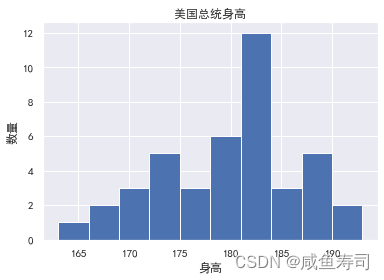
前25%身高: 183.0
平均值: 179.73809523809524
中位数: 182.0
方差: 48.05045351473922
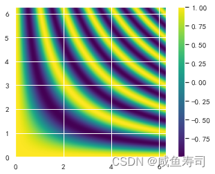
广播

因为只会在左边补维度,因此想要不报错可以自行在右边用newaxis添加维度
import numpy as np
import matplotlib.pyplot as plt
x = np.linspace(0, 2*np.pi, 100)
y = np.linspace(0, 2*np.pi, 100)[:,np.newaxis]
# 其实也可以使用z = np.cos(np.multiply.outer(x, x))
z = np.cos(x*y)
plt.imshow(z, cmap='viridis', extent=[0, 2*np.pi, 0, 2*np.pi], origin='lower')
plt.colorbar()
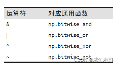
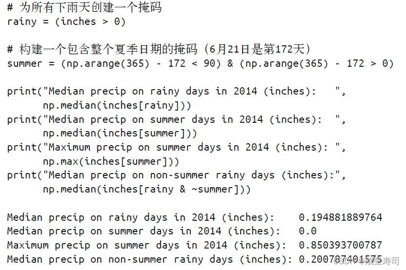
比较,掩码与布尔逻辑
import numpy as np
heights = np.array([189, 170, 189, 163, 183, 171, 185, 168, 173, 183, 173, 173, 175, 178, 183, 193, 178, 173,
174, 183, 183, 168, 170, 178, 182, 180, 183, 178, 182, 188, 175, 179, 183, 193, 182, 183,
177, 185, 188, 188, 182, 185])
block = heights > 180
print(heights > 180)
print("有{}位总统身高大于180".format(np.sum(block)))
print("是否有总统身高小于165:",np.any(block))
print("是否所有总统身高大于165:",np.all(block))
print(heights[heights > 180])
[ True False True False True False True False False True False False
False False True True False False False True True False False False
True False True False True True False False True True True True
False True True True True True]
有22位总统身高大于180
是否有总统身高小于165: True
是否所有总统身高大于165: False
[189 189 183 185 183 183 193 183 183 182 183 182 188 183 193 182 183 185
188 188 182 185]
除了比较,也可以使用布尔运算符
花哨索引
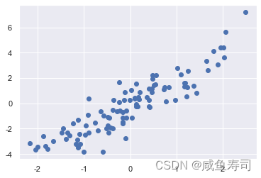
# In[11]
import numpy as np
import matplotlib.pyplot as plt
import seaborn
seaborn.set()
np.random.seed(114514)
mean = [0, 0]
cov = [[1, 2], [2, 5]]
a = np.random.multivariate_normal(mean, cov, 100)
print(a.shape)
plt.scatter(a[:,0], a[:,1])
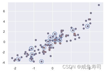
indices = np.random.randint(0, 100, 20)
print(indices)
selection = a[indices]
print(selection.shape)
plt.scatter(a[:, 0], a[:, 1], alpha=0.3)
plt.scatter(selection[:, 0], selection[:, 1], facecolor='none', edgecolor='b', s=200)(100, 2)
[74 5 37 74 40 37 95 82 11 28 38 50 24 28 96 31 92 48 47 10]
(20, 2)
可以使用用花哨的索引修改值
注意如果索引包含多个相同值,想要完成修改值需要使用at方法
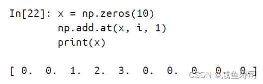
import numpy as np
import matplotlib.pyplot as plt
np.random.seed(42)
x = np.random.randn(100)
# 手动计算直方图
bins = np.linspace(-5, 5, 20)
counts = np.zeros_like(bins)
# 为每个x找到合适的区间
i = np.searchsorted(bins, x)
# 为每个区间加上1
np.add.at(counts, i, 1)
plt.plot(bins, counts)
也可以使用plt.hist(x, bins, histtype='step')达成相同的效果
x[:-1] > x[1:]可以比较数组前一位和后一位,太巧妙了
排序
np.sort()返回排序结果,参数axis可以指定排序维度
np.argsoet()返回排序的索引
np.partition()
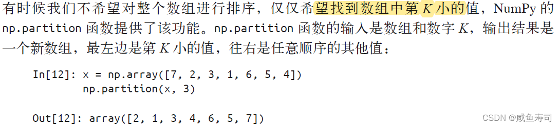
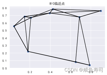
import numpy as np
import matplotlib.pyplot as plt
import seaborn
seaborn.set()
plt.rcParams['font.sans-serif'] = ['SimHei']  # 用来正常显示中文标签
plt.rcParams['axes.unicode_minus'] = False  # 用来正常显示负号`
K = 3
np.random.seed(114514)
# 在均匀分布中选取十个点
X = np.random.rand(10,2)
# 获取所有点的平方差的矩阵
difference = np.sum(np.power((X[np.newaxis,:,:]-X[:,np.newaxis,:]), 2), axis=-1)
# 按照近远每行进行排序
nearest = np.argsort(difference, axis=1)
nearest_3 = nearest[:,:K+1]
plt.scatter(X[:,0], X[:,1])
# 十行
for i in range(X.shape[0]):
    for j in nearest_3[i, :K+1]:
    # 画一条从X[i]到X[j]的线段
    # 用zip方法实现:
        plt.plot(*zip(X[j], X[i]), color='black')
        plt.title(f"K={K}临近点")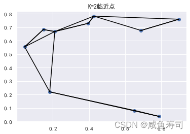
结构化数据
结构化数据可以修改numpy数组的元素类型,通过np.dtype实现
两种方法:
1.使用字典

2.使用元组
![]()
numpy的数据类型
通过view和np.recarry方法可以获得数组的视图,这样访问时就把key变成了数组的属性
import numpy as np
type = np.dtype([('name','S10'),('age','<i4'),('instrument','S10')])
mygo = np.zeros(5, dtype=type)
names = np.array(["tomorin","rana","ano","rikki","soyorin"])
ages = np.array([16, 15, 16, 16, 16])
ages = ages[np.newaxis, :]
instruments = np.array(["microphone","guitar","guitar","drum","base"])

mygo['name'] = names
mygo['age'] = ages
mygo['instrument'] = instruments

mygo_view = mygo.view(np.recarray)
print(mygo_view.name)
print(mygo[mygo['age'] >= 16]['name'])
[b'tomorin' b'rana' b'ano' b'rikki' b'soyorin']
[b'tomorin' b'ano' b'rikki' b'soyorin']


 被折叠的 条评论
为什么被折叠?
被折叠的 条评论
为什么被折叠?
 到【灌水乐园】发言


