


配置环境
①首先打开 cmd,创建虚拟环境。
conda create -n tf1 python=3.6
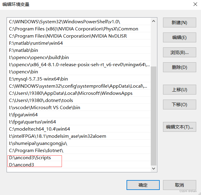
如果报错:‘conda’ 不是内部或外部命令,也不是可运行的程序 或批处理文件。请在环境变量里添加Anconda3路径,如果没有Anconda3直接去官网下载就行了
具体步骤:我的电脑—右键属性—高级系统设置—环境变量—系统变量—Path—双击进入—新建—浏览—找到Anaconda和Scripts的路径添加,然后点击确定就好了。
②激活环境
activate
conda activate tf1
③安装 tensorflow、keras 库。
pip install tensorflow==1.14.0 -i “https://pypi.doubanio.com/simple/”
pip install keras==2.2.5 -i “https://pypi.doubanio.com/simple/”
④安装 nb_conda_kernels 包。
conda install nb_conda_kernels
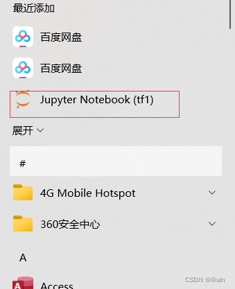
⑤打开 Jupyter Notebook(tf1)按win查看
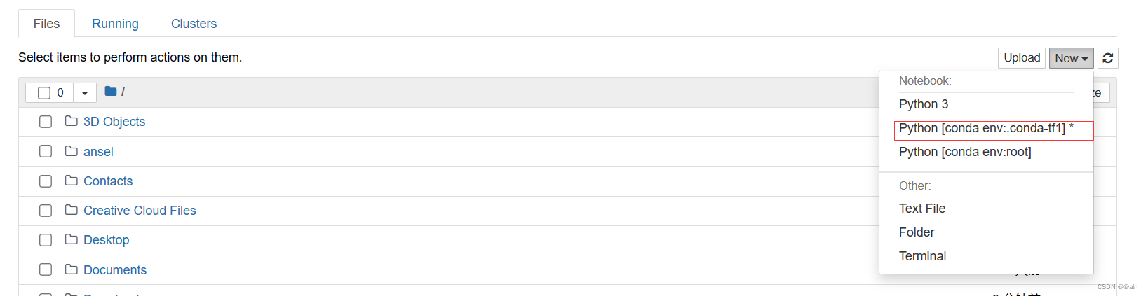
⑥点击【New】→【Python[tf1环境下的]】创建 python 文件。
猫狗数据分类建模
①下载猫狗数据
链接:https://pan.baidu.com/s/1nIDrl3ZFZCMpHzD3OmN7Mg
提取码:7vjj
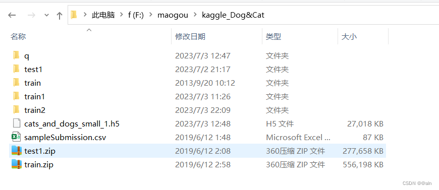
下载完毕后,将其解压在无中文的目录下
②对猫狗图像进行分类
import os, shutil
# 原始目录所在的路径
original_dataset_dir = 'F:\\maogou\\kaggle_Dog&Cat\\train\\'

# 数据集分类后的目录
base_dir = 'F:\\maogou\\kaggle_Dog&Cat\\train1\\'
os.mkdir(base_dir)

# # 训练、验证、测试数据集的目录
train_dir = os.path.join(base_dir, 'train')
os.mkdir(train_dir)
validation_dir = os.path.join(base_dir, 'validation')
os.mkdir(validation_dir)
test_dir = os.path.join(base_dir, 'test')
os.mkdir(test_dir)

# 猫训练图片所在目录
train_cats_dir = os.path.join(train_dir, 'cats')
os.mkdir(train_cats_dir)

# 狗训练图片所在目录
train_dogs_dir = os.path.join(train_dir, 'dogs')
os.mkdir(train_dogs_dir)

# 猫验证图片所在目录
validation_cats_dir = os.path.join(validation_dir, 'cats')
os.mkdir(validation_cats_dir)

# 狗验证数据集所在目录
validation_dogs_dir = os.path.join(validation_dir, 'dogs')
os.mkdir(validation_dogs_dir)

# 猫测试数据集所在目录
test_cats_dir = os.path.join(test_dir, 'cats')
os.mkdir(test_cats_dir)

# 狗测试数据集所在目录
test_dogs_dir = os.path.join(test_dir, 'dogs')
os.mkdir(test_dogs_dir)

# 将前1000张猫图像复制到train_cats_dir
fnames = ['cat.{}.jpg'.format(i) for i in range(1000)]
for fname in fnames:
    src = os.path.join(original_dataset_dir, fname)
    dst = os.path.join(train_cats_dir, fname)
    shutil.copyfile(src, dst)

# 将下500张猫图像复制到validation_cats_dir
fnames = ['cat.{}.jpg'.format(i) for i in range(1000, 1500)]
for fname in fnames:
    src = os.path.join(original_dataset_dir, fname)
    dst = os.path.join(validation_cats_dir, fname)
    shutil.copyfile(src, dst)

# 将下500张猫图像复制到test_cats_dir
fnames = ['cat.{}.jpg'.format(i) for i in range(1500, 2000)]
for fname in fnames:
    src = os.path.join(original_dataset_dir, fname)
    dst = os.path.join(test_cats_dir, fname)
    shutil.copyfile(src, dst)

# 将前1000张狗图像复制到train_dogs_dir
fnames = ['dog.{}.jpg'.format(i) for i in range(1000)]
for fname in fnames:
    src = os.path.join(original_dataset_dir, fname)
    dst = os.path.join(train_dogs_dir, fname)
    shutil.copyfile(src, dst)

# 将下500张狗图像复制到validation_dogs_dir
fnames = ['dog.{}.jpg'.format(i) for i in range(1000, 1500)]
for fname in fnames:
    src = os.path.join(original_dataset_dir, fname)
    dst = os.path.join(validation_dogs_dir, fname)
    shutil.copyfile(src, dst)

# 将下500张狗图像复制到test_dogs_dir
fnames = ['dog.{}.jpg'.format(i) for i in range(1500, 2000)]
for fname in fnames:
    src = os.path.join(original_dataset_dir, fname)
    dst = os.path.join(test_dogs_dir, fname)
    shutil.copyfile(src, dst)
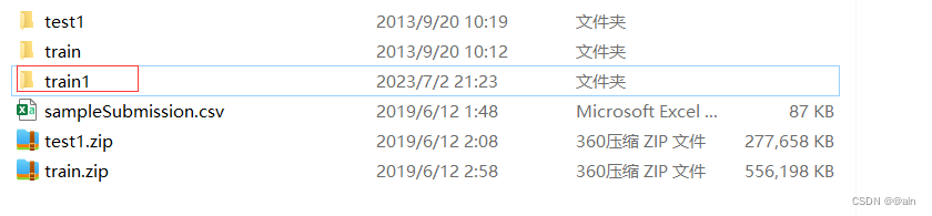
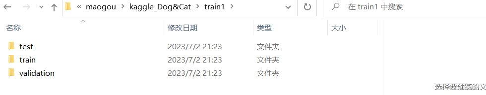
处理后新加了一个train文件
③查看分类后,对应目录下的图片数量:
#输出数据集对应目录下图片数量
print('total training cat images:', len(os.listdir(train_cats_dir)))
print('total training dog images:', len(os.listdir(train_dogs_dir)))
print('total validation cat images:', len(os.listdir(validation_cats_dir)))
print('total validation dog images:', len(os.listdir(validation_dogs_dir)))
print('total test cat images:', len(os.listdir(test_cats_dir)))
print('total test dog images:', len(os.listdir(test_dogs_dir)))
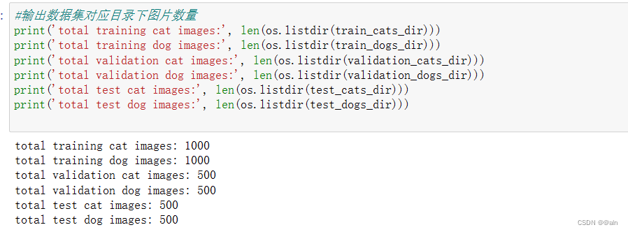
(猫狗训练图片各 1000 张,验证图片各 500 张,测试图片各 500 张。)
猫狗分类的实例基准模型
①构建网络模型:
先更新一下numpy
pip install numpy==1.16.4 -i "https://pypi.doubanio.com/simple/"
构建
#网络模型构建
from keras import layers
from keras import models
#keras的序贯模型
model = models.Sequential()
#卷积层,卷积核是3*3,激活函数relu
model.add(layers.Conv2D(32, (3, 3), activation='relu',
                        input_shape=(150, 150, 3)))
#最大池化层
model.add(layers.MaxPooling2D((2, 2)))
#卷积层,卷积核2*2,激活函数relu
model.add(layers.Conv2D(64, (3, 3), activation='relu'))
#最大池化层
model.add(layers.MaxPooling2D((2, 2)))
#卷积层,卷积核是3*3,激活函数relu
model.add(layers.Conv2D(128, (3, 3), activation='relu'))
#最大池化层
model.add(layers.MaxPooling2D((2, 2)))
#卷积层,卷积核是3*3,激活函数relu
model.add(layers.Conv2D(128, (3, 3), activation='relu'))
#最大池化层
model.add(layers.MaxPooling2D((2, 2)))
#flatten层,用于将多维的输入一维化,用于卷积层和全连接层的过渡
model.add(layers.Flatten())
#全连接,激活函数relu
model.add(layers.Dense(512, activation='relu'))
#全连接,激活函数sigmoid
model.add(layers.Dense(1, activation='sigmoid'))
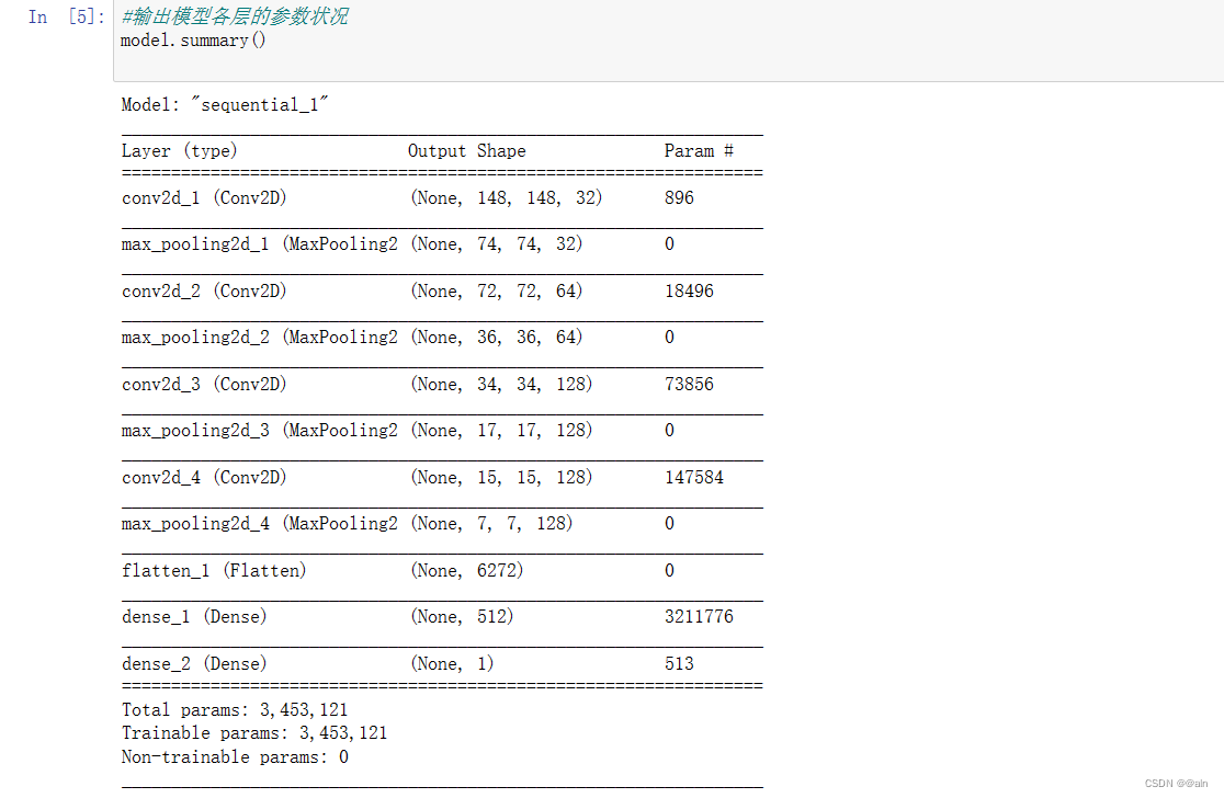
查看模型各层的参数状况
#输出模型各层的参数状况
model.summary()
②配置优化器
- loss:计算损失,这里用的是交叉熵损失
metrics:列表,包含评估模型在训练和测试时的性能的指标
from keras import optimizers

model.compile(loss='binary_crossentropy',
              optimizer=optimizers.RMSprop(lr=1e-4),
              metrics=['acc'])
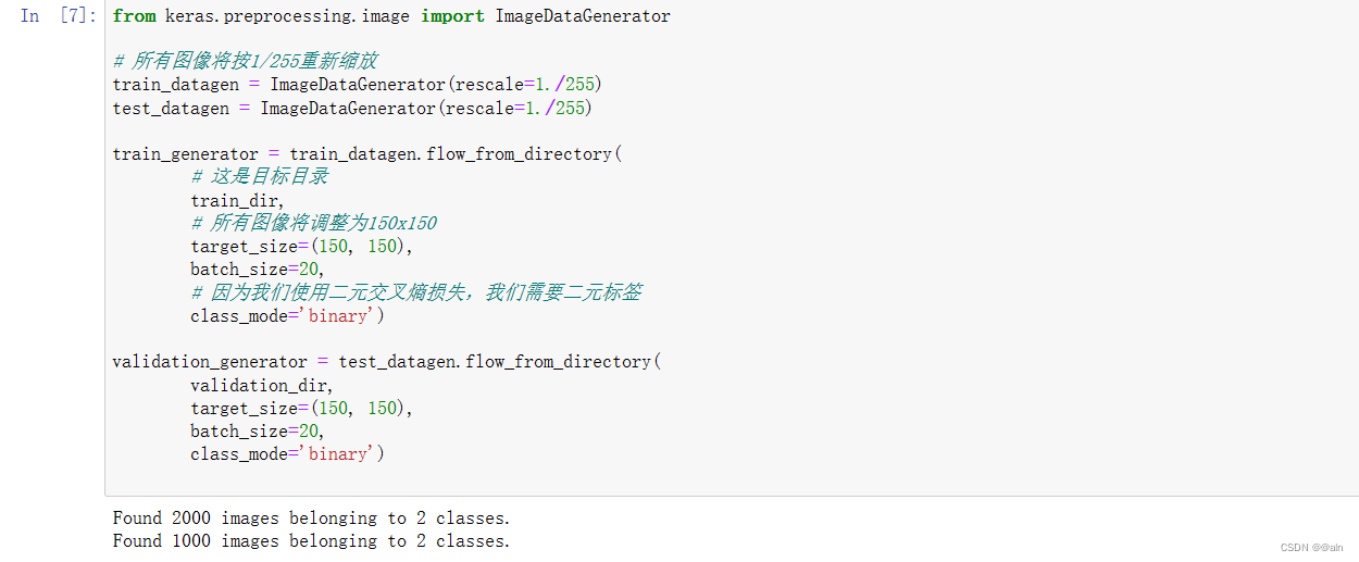
③图片格式转化
- 所有图片(2000张)重设尺寸大小为 150x150 大小,并使用 ImageDataGenerator 工具将本地图片 .jpg 格式转化成 RGB 像素网格,再转化成浮点张量上传到网络上。
from keras.preprocessing.image import ImageDataGenerator

# 所有图像将按1/255重新缩放
train_datagen = ImageDataGenerator(rescale=1./255)
test_datagen = ImageDataGenerator(rescale=1./255)

train_generator = train_datagen.flow_from_directory(
        # 这是目标目录
        train_dir,
        # 所有图像将调整为150x150
        target_size=(150, 150),
        batch_size=20,
        # 因为我们使用二元交叉熵损失,我们需要二元标签
        class_mode='binary')

validation_generator = test_datagen.flow_from_directory(
        validation_dir,
        target_size=(150, 150),
        batch_size=20,
        class_mode='binary')
- 查看上述图像预处理过程中生成器的输出
先安装 pillow 库
pip install pillow -i “https://pypi.doubanio.com/simple/”
查看
#查看上面对于图片预处理的处理结果
for data_batch, labels_batch in train_generator:
    print('data batch shape:', data_batch.shape)
    print('labels batch shape:', labels_batch.shape)
    break
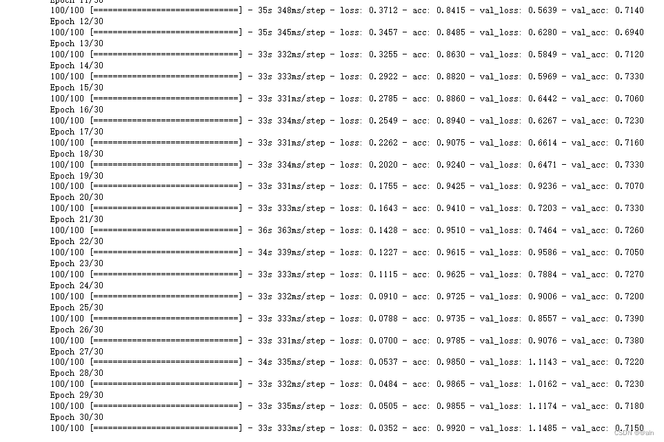
④开始训练模型
#模型训练过程
history = model.fit_generator(
      train_generator,
      steps_per_epoch=100,
      epochs=30,
      validation_data=validation_generator,
      validation_steps=50)
⑤保存模型,结果可视化
保存模型
#保存训练得到的的模型
model.save('F:\\maogou\\kaggle_Dog&Cat\\cats_and_dogs_small_1.h5')

可视化
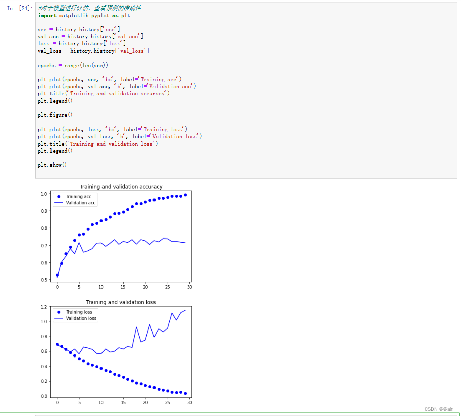
#对于模型进行评估,查看预测的准确性
import matplotlib.pyplot as plt

acc = history.history['acc']
val_acc = history.history['val_acc']
loss = history.history['loss']
val_loss = history.history['val_loss']

epochs = range(len(acc))

plt.plot(epochs, acc, 'bo', label='Training acc')
plt.plot(epochs, val_acc, 'b', label='Validation acc')
plt.title('Training and validation accuracy')
plt.legend()

plt.figure()

plt.plot(epochs, loss, 'bo', label='Training loss')
plt.plot(epochs, val_loss, 'b', label='Validation loss')
plt.title('Training and validation loss')
plt.legend()

plt.show()
⑥结果分析
- 很明显模型上来就过拟合了,主要原因是数据不够,或者说相对于数据量,模型过复杂(训练损失在第30个epoch就降为0了),训练精度随着时间线性增长,直到接近100%,而我们的验证精度停留在70-72%。我们的验证损失在5个epoch后达到最小,然后停止,而训练损失继续线性下降,直到接近0。
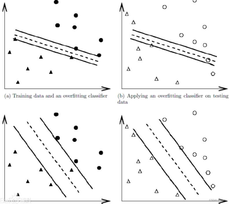
- 过拟合的定义: 给定一个假设空间 H HH,一个假设 h hh 属于 H HH,如果存在其他的假设 h ’ h’h’ 属于 H HH,使得在训练样例上 h hh 的错误率比 h ’ h’h’ 小,但在整个实例分布上 h ’ h’h’ 比 h hh 的错误率小,那么就说假设 h hh 过度拟合训练数据。
举个简单的例子,( a )( b )过拟合,( c )( d )不过拟合,如下图所示:
- 过拟合常见解决方法:
(1)在神经网络模型中,可使用权值衰减的方法,即每次迭代过程中以某个小因子降低每个权值。
(2)选取合适的停止训练标准,使对机器的训练在合适的程度;
(3)保留验证数据集,对训练成果进行验证;
(4)获取额外数据进行交叉验证;
(5)正则化,即在进行目标函数或代价函数优化时,在目标函数或代价函数后面加上一个正则项,一般有L1正则与L2正则等。 - 不过接下来将使用一种新的方法,专门针对计算机视觉,在深度学习模型处理图像时几乎普遍使用——数据增强。
猫狗分类的实例基准模型之数据增强
①数据增强定义
- 数据集增强主要是为了减少网络的过拟合现象,通过对训练图片进行变换可以得到泛化能力更强的网络,更好的适应应用场景。
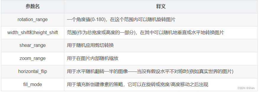
- 常用的数据增强方法有:
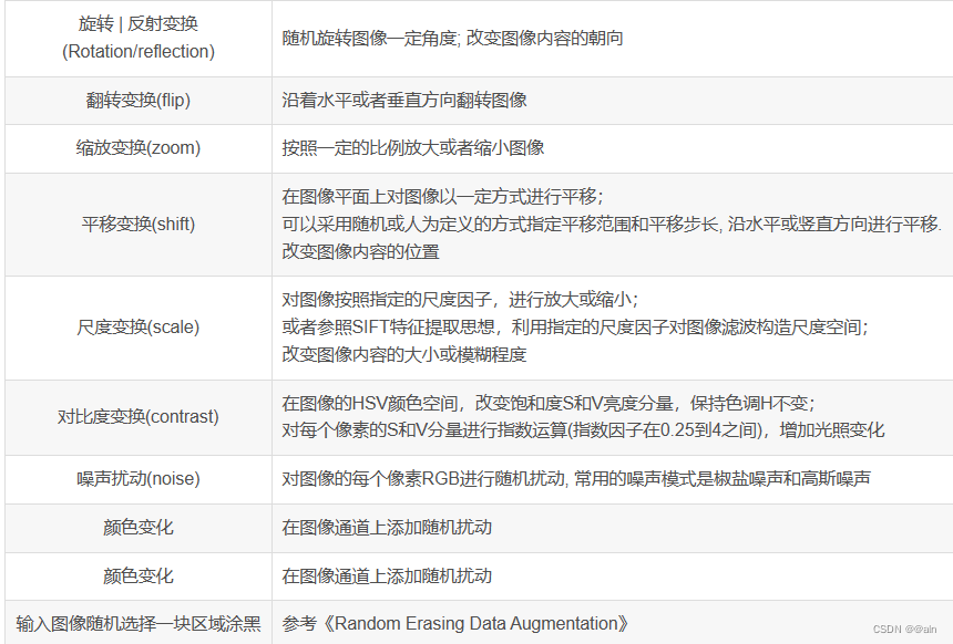
②重新构建模型:
-
上面建完的模型就保留着,我们重新建一个 .ipynb 文件,重新开始建模。
-
首先猫狗图像预处理,只不过这里将分类好的数据集放在 train2 文件夹中,其它的都一样。

-
然后配置网络模型、构建优化器,然后进行数据增强,代码如下:
from keras.preprocessing.image import ImageDataGenerator
datagen = ImageDataGenerator(
      rotation_range=40,
      width_shift_range=0.2,
      height_shift_range=0.2,
      shear_range=0.2,
      zoom_range=0.2,
      horizontal_flip=True,
      fill_mode='nearest')
- 参数解释:
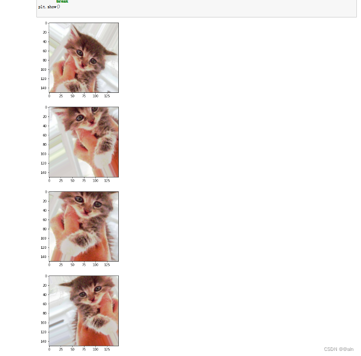
- 查看数据增强后的效果:
import matplotlib.pyplot as plt
# This is module with image preprocessing utilities
from keras.preprocessing import image
fnames = [os.path.join(train_cats_dir, fname) for fname in os.listdir(train_cats_dir)]
# We pick one image to "augment"
img_path = fnames[3]
# Read the image and resize it
img = image.load_img(img_path, target_size=(150, 150))
# Convert it to a Numpy array with shape (150, 150, 3)
x = image.img_to_array(img)
# Reshape it to (1, 150, 150, 3)
x = x.reshape((1,) + x.shape)
# The .flow() command below generates batches of randomly transformed images.
# It will loop indefinitely, so we need to `break` the loop at some point!
i = 0
for batch in datagen.flow(x, batch_size=1):
    plt.figure(i)
    imgplot = plt.imshow(image.array_to_img(batch[0]))
    i += 1
    if i % 4 == 0:
        break
plt.show()
- 结果如下
- 图片格式转化
train_datagen = ImageDataGenerator(
    rescale=1./255,
    rotation_range=40,
    width_shift_range=0.2,
    height_shift_range=0.2,
    shear_range=0.2,
    zoom_range=0.2,
    horizontal_flip=True,)
# Note that the validation data should not be augmented!
test_datagen = ImageDataGenerator(rescale=1./255)
train_generator = train_datagen.flow_from_directory(
        # This is the target directory
        train_dir,
        # All images will be resized to 150x150
        target_size=(150, 150),
        batch_size=32,
        # Since we use binary_crossentropy loss, we need binary labels
        class_mode='binary')
validation_generator = test_datagen.flow_from_directory(
        validation_dir,
        target_size=(150, 150),
        batch_size=32,
        class_mode='binary')
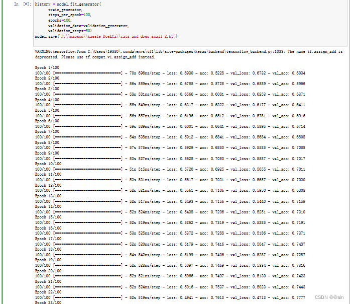
- 开始训练并保存结果
history = model.fit_generator(
      train_generator,
      steps_per_epoch=100,
      epochs=100,
      validation_data=validation_generator,
      validation_steps=50)
model.save('E:\\Cat_And_Dog\\kaggle\\cats_and_dogs_small_2.h5')
-
训练结果如下
-
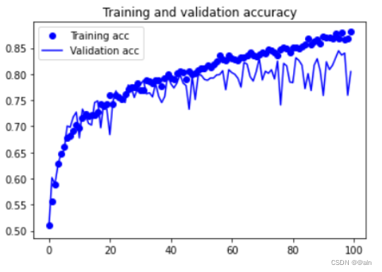
结果可视化
acc = history.history['acc']
val_acc = history.history['val_acc']
loss = history.history['loss']
val_loss = history.history['val_loss']
epochs = range(len(acc))
plt.plot(epochs, acc, 'bo', label='Training acc')
plt.plot(epochs, val_acc, 'b', label='Validation acc')
plt.title('Training and validation accuracy')
plt.legend()
plt.figure()
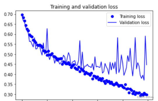
plt.plot(epochs, loss, 'bo', label='Training loss')
plt.plot(epochs, val_loss, 'b', label='Validation loss')
plt.title('Training and validation loss')
plt.legend()
plt.show()
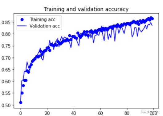
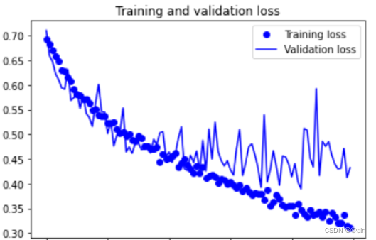
③dropout层定义及添加实现
- 在数据增强的基础上,再添加一个 dropout 层。
#退出层
model.add(layers.Dropout(0.5))
- 再次训练模型,查看训练结果如下
问题回答
①什么是overfit(过拟合)?
过拟合(overfitting)是指机器学习算法在训练数据上表现出很高的准确性,但在未见过的测试数据上表现较差的现象。简而言之,过拟合就是模型过度适应了训练数据,导致在面对新数据时泛化能力较差。当一个机器学习模型过拟合时,它会记住训练数据中的细节和噪声,而不是学习到普遍适用的模式。这种现象可能发生在模型的复杂性过高、训练数据数量不足或数据中存在噪声等情况下。
②什么是数据增强?
数据增强(data augmentation)是一种在机器学习和深度学习中常用的技术,用于通过对原始训练数据进行变换和扩充来增加数据样本的数量。数据增强旨在改变训练数据的外观,但保持其标签和语义不变,从而提供更多样化、更丰富的数据样本,以改善模型的泛化能力。
数据增强可以通过多种方式进行操作,包括但不限于以下方法:
镜像翻转:将图像水平或垂直翻转,产生左右或上下镜像的图像。
旋转:对图像进行旋转操作,如随机旋转一定角度。
平移:在图像上进行平移操作,将图像在水平或垂直方向上移动一定距离。
缩放:对图像进行缩放操作,放大或缩小图像的尺寸。
裁剪:从原始图像中裁剪出感兴趣的区域,改变图像的大小和内容。
增加噪声:向图像中添加噪声,如高斯噪声、椒盐噪声等。
亮度和对比度调整:调整图像的亮度和对比度,改变图像的整体明暗程度。
颜色变换:对图像进行颜色空间的变换,如灰度化、色彩偏移等。
③如果单独只做数据增强,精确率提高了多少?
由于数据量的增加,对比基准模型,可以很明显的观察到曲线没有过度拟合了,训练曲线紧密地跟踪验证曲线,这也就是数据增强带来的影响,但是可以发现它的波动幅度还是比较大的。
④再添加的dropout层,是什么实际效果?
相比于只使用数据增强的效果来看,额外添加一层 dropout 层,仔细对比,可以发现训练曲线更加紧密地跟踪验证曲线,波动的幅度也降低了些,训练效果更棒了。


 196
196


 被折叠的 条评论
为什么被折叠?
被折叠的 条评论
为什么被折叠?
 到【灌水乐园】发言


