机器学习实战(1)--回归分析

写在前面的话：纯粹标题党了，今天上完课，来总结一下老师讲的，文末附数据。以下展示代码均基于IDLE或者jupyter notebook
文章将分为以下部分

1. 读入数据
2. 线性回归
3. 多项式回归
4. 结果校验

环境配置：

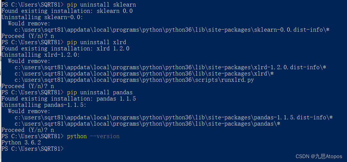
读入数据

首先是读入数据，由于我的文件是excel格式的，请读入的时候使用pandas的read_excel读入，不要用read_csv读入。
参考：这里

#fpath为excel的绝对路径
>>>df=pd.read_excel(fpath)
>>>df.head(5)
   year  price
0   0.0  10808
1   0.1  13611
2   0.2  12306
3   0.3  12151
4   0.3  13057

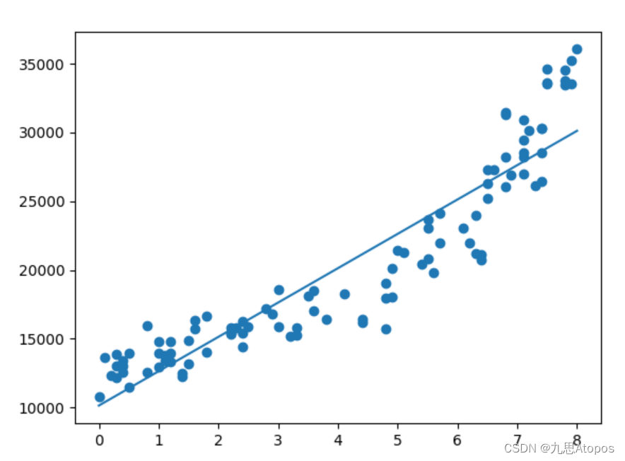
线性回归

我们使用的是sklearn的LinearRegression函数，具体注意的细节为输入x是二维的DataFrame形式。我们以year为自变量x，以price为因变量y，构造二维的x又以下两种方式：
方法1：

>>> x=df['year']
>>> x
0     0.0
1     0.1
2     0.2
3     0.3
4     0.3
     ... 
95    7.8
96    7.8
97    7.9
98    7.9
99    8.0
Name: year, Length: 100, dtype: float64
>>> x.size
100
>>> a=[[x[i]] for i in range(x.size)]
>>> a
[[0.0], [0.1], [0.2], [0.3], [0.3], [0.3], [0.4], [0.4], [0.4], [0.5], [0.5], [0.8], [0.8], [1.0], [1.0], [1.0], [1.1], [1.1], [1.2], [1.2], [1.2], [1.4], [1.4], [1.5], [1.5], [1.6], [1.6], [1.8], [1.8], [2.2], [2.2], [2.2], [2.3], [2.4], [2.4], [2.4], [2.5], [2.8], [2.9], [3.0], [3.0], [3.2], [3.3], [3.3], [3.5], [3.6], [3.6], [3.8], [4.1], [4.4], [4.4], [4.8], [4.8], [4.8], [4.9], [4.9], [5.0], [5.1], [5.4], [5.5], [5.5], [5.5], [5.6], [5.7], [5.7], [6.1], [6.2], [6.3], [6.3], [6.4], [6.4], [6.5], [6.5], [6.5], [6.6], [6.8], [6.8], [6.8], [6.8], [6.9], [7.1], [7.1], [7.1], [7.1], [7.1], [7.2], [7.3], [7.4], [7.4], [7.4], [7.4], [7.5], [7.5], [7.5], [7.8], [7.8], [7.8], [7.9], [7.9], [8.0]]
>>> 

方法2：

>>> x=df[['year']]
>>> x
    year
0    0.0
1    0.1
2    0.2
3    0.3
4    0.3
..   ...
95   7.8
96   7.8
97   7.9
98   7.9
99   8.0

[100 rows x 1 columns]
>>> 

线性拟合:
原理说明：这里

from sklearn.linear_model import LinearRegression
>>> r=LinearRegression()
>>> r.fit(x,y)

结果展示：

>>> y=df['price']
>>> r.fit(x,y)
LinearRegression()

>>> import matplotlib.pyplot as plt
>>> plt.scatter(x,y)
<matplotlib.collections.PathCollection object at 0x000002A88DE13978>
>>> plt.plot(x,r.predict(x))
[<matplotlib.lines.Line2D object at 0x000002A88DE13CC0>]
>>> plt.show()

多项式回归

思路：对$x$做变换为$[1,x,x^2]$，之后进行$x$和$y$的线性回归。
做变换：

>>> from sklearn.preprocessing import PolynomialFeatures as pf
>>> pl=pf()
>>> pl=pf(degree=2)
>>> x=pl.fit_transform(x)
>>> x
array([[1.000e+00, 0.000e+00, 0.000e+00],
       [1.000e+00, 1.000e-01, 1.000e-02],
       [1.000e+00, 2.000e-01, 4.000e-02],
       [1.000e+00, 3.000e-01, 9.000e-02],
       [1.000e+00, 3.000e-01, 9.000e-02],
       [1.000e+00, 3.000e-01, 9.000e-02],

线性回归：

>>> r
LinearRegression()
>>> r.fit(x,y)
LinearRegression()
>>> plt.scatter(df['year'],y)
<matplotlib.collections.PathCollection object at 0x000002A88C6F5860>
>>> plt.plot(df['year'],r.predict(x),color='red')
[<matplotlib.lines.Line2D object at 0x000002A88DE30668>]
>>> plt.show()

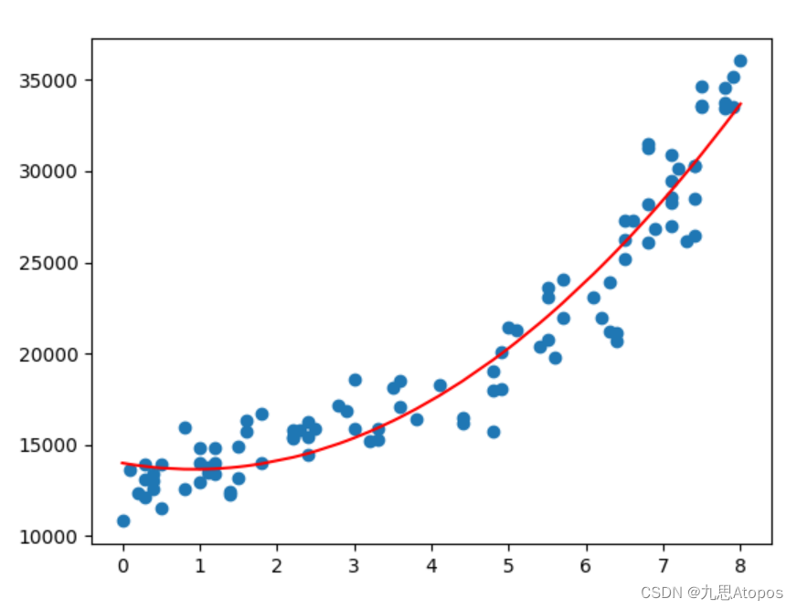
结果验证：

>>> sklearn.metrics.r2_score(y,r.predict(x))
0.9310387116075501
>>> 

查看参数

>>> r.coef_#w
array([   0.        , -743.68080444,  400.80398224])
>>> r.intercept_#b
13988.159332096888
>>> 

数据：

链接：https://pan.baidu.com/s/1GdZr31ZzHUZQyRbdwr-iiw?pwd=1234
提取码：1234

未展示但可能对您有用的全部代码(含报错）

链接：https://pan.baidu.com/s/1bt0VgtA0vqYBoKt6KkOoLw?pwd=1234
提取码：1234