


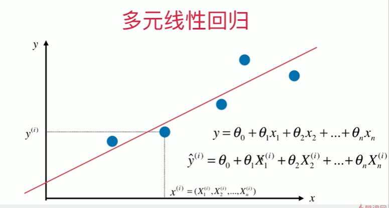
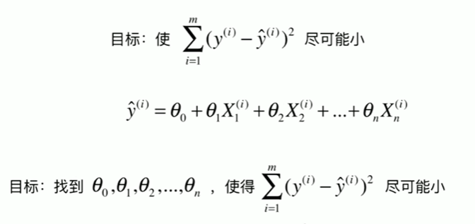
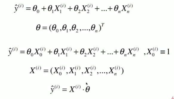
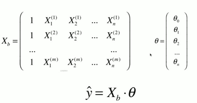
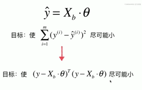
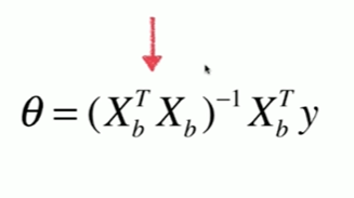
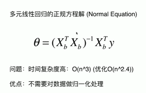
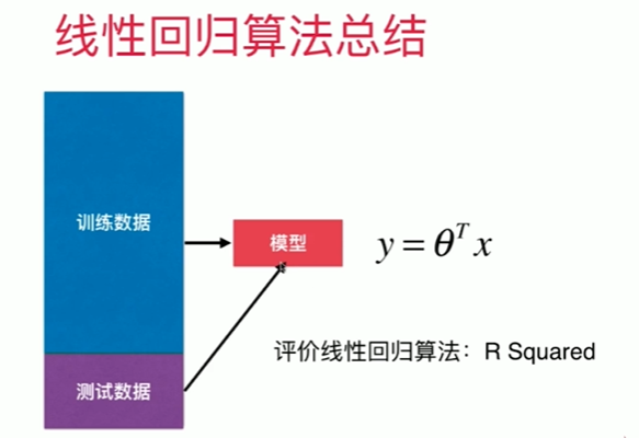
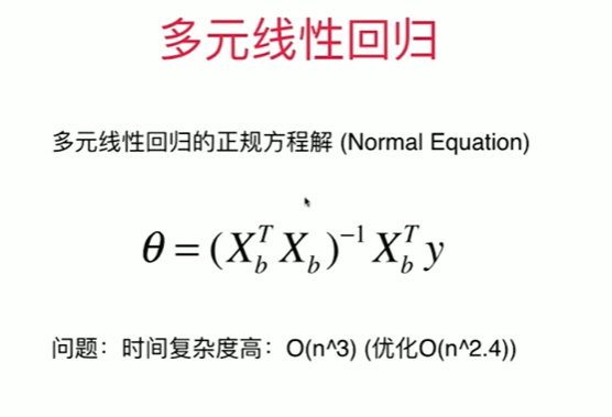
5-7 多元线性回归和正规方程解
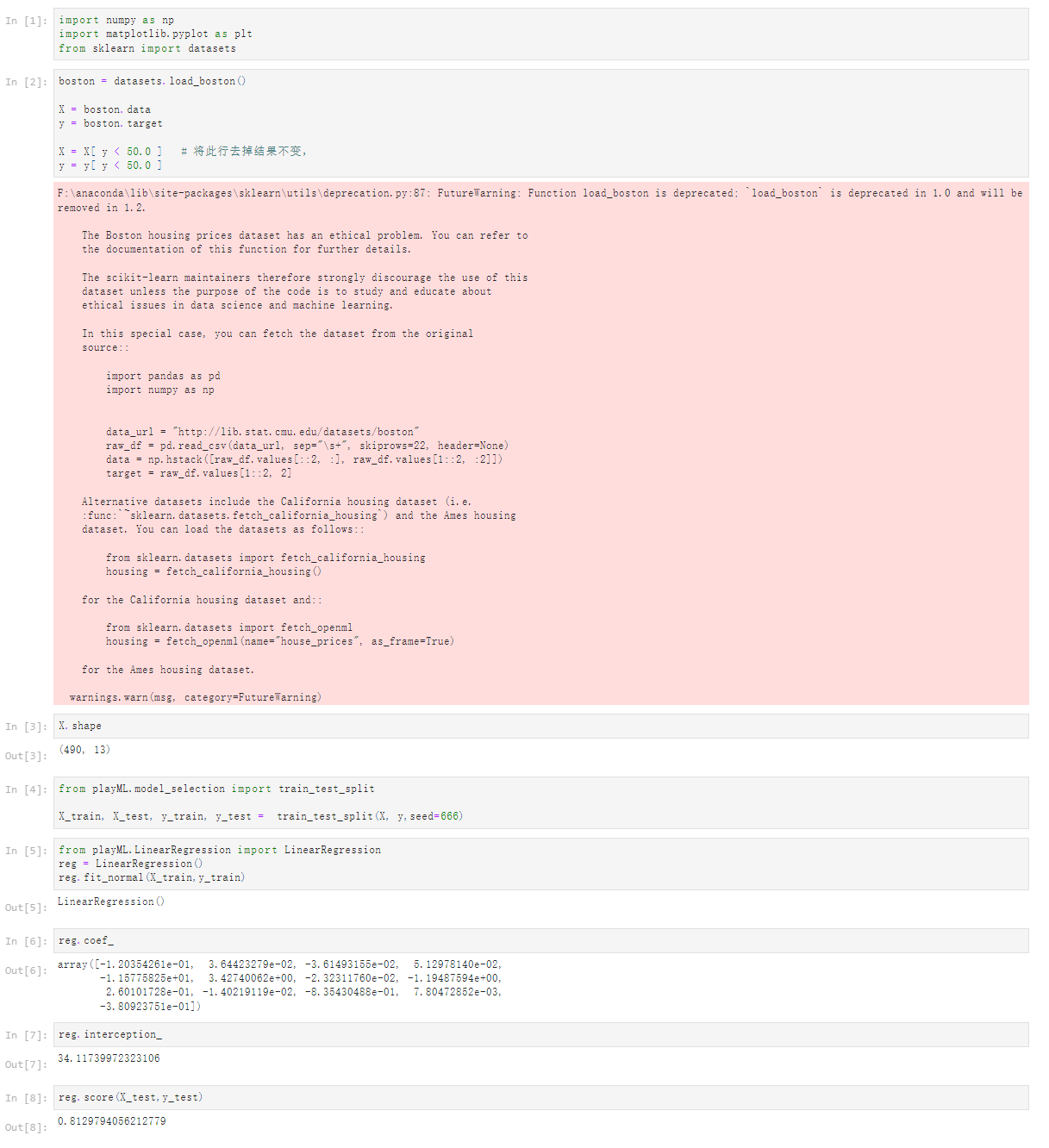
5-8 实现多元线性回归

Notbook 示例
Notbook 源码
[1]
import numpy as np
import matplotlib.pyplot as plt
from sklearn import datasets
[2]
boston = datasets.load_boston()

X = boston.data
y = boston.target

X = X[ y < 50.0 ]   # 将此行去掉结果不变,
y = y[ y < 50.0 ]
F:\anaconda\lib\site-packages\sklearn\utils\deprecation.py:87: FutureWarning: Function load_boston is deprecated; `load_boston` is deprecated in 1.0 and will be removed in 1.2.

    The Boston housing prices dataset has an ethical problem. You can refer to
    the documentation of this function for further details.

    The scikit-learn maintainers therefore strongly discourage the use of this
    dataset unless the purpose of the code is to study and educate about
    ethical issues in data science and machine learning.

    In this special case, you can fetch the dataset from the original
    source::

        import pandas as pd
        import numpy as np


        data_url = "http://lib.stat.cmu.edu/datasets/boston"
        raw_df = pd.read_csv(data_url, sep="\s+", skiprows=22, header=None)
        data = np.hstack([raw_df.values[::2, :], raw_df.values[1::2, :2]])
        target = raw_df.values[1::2, 2]

    Alternative datasets include the California housing dataset (i.e.
    :func:`~sklearn.datasets.fetch_california_housing`) and the Ames housing
    dataset. You can load the datasets as follows::

        from sklearn.datasets import fetch_california_housing
        housing = fetch_california_housing()

    for the California housing dataset and::

        from sklearn.datasets import fetch_openml
        housing = fetch_openml(name="house_prices", as_frame=True)

    for the Ames housing dataset.

  warnings.warn(msg, category=FutureWarning)

[3]
X.shape
(490, 13)
[4]
from playML.model_selection import train_test_split

X_train, X_test, y_train, y_test =  train_test_split(X, y,seed=666)
[5]
from playML.LinearRegression import LinearRegression
reg = LinearRegression()
reg.fit_normal(X_train,y_train)
LinearRegression()
[6]
reg.coef_
array([-1.20354261e-01,  3.64423279e-02, -3.61493155e-02,  5.12978140e-02,
       -1.15775825e+01,  3.42740062e+00, -2.32311760e-02, -1.19487594e+00,
        2.60101728e-01, -1.40219119e-02, -8.35430488e-01,  7.80472852e-03,
       -3.80923751e-01])
[7]
reg.interception_
34.11739972323106
[8]
reg.score(X_test,y_test)
0.8129794056212779
5-9 使用scikit-learn解决回归问题
Notbook 示例
Notbook 源码
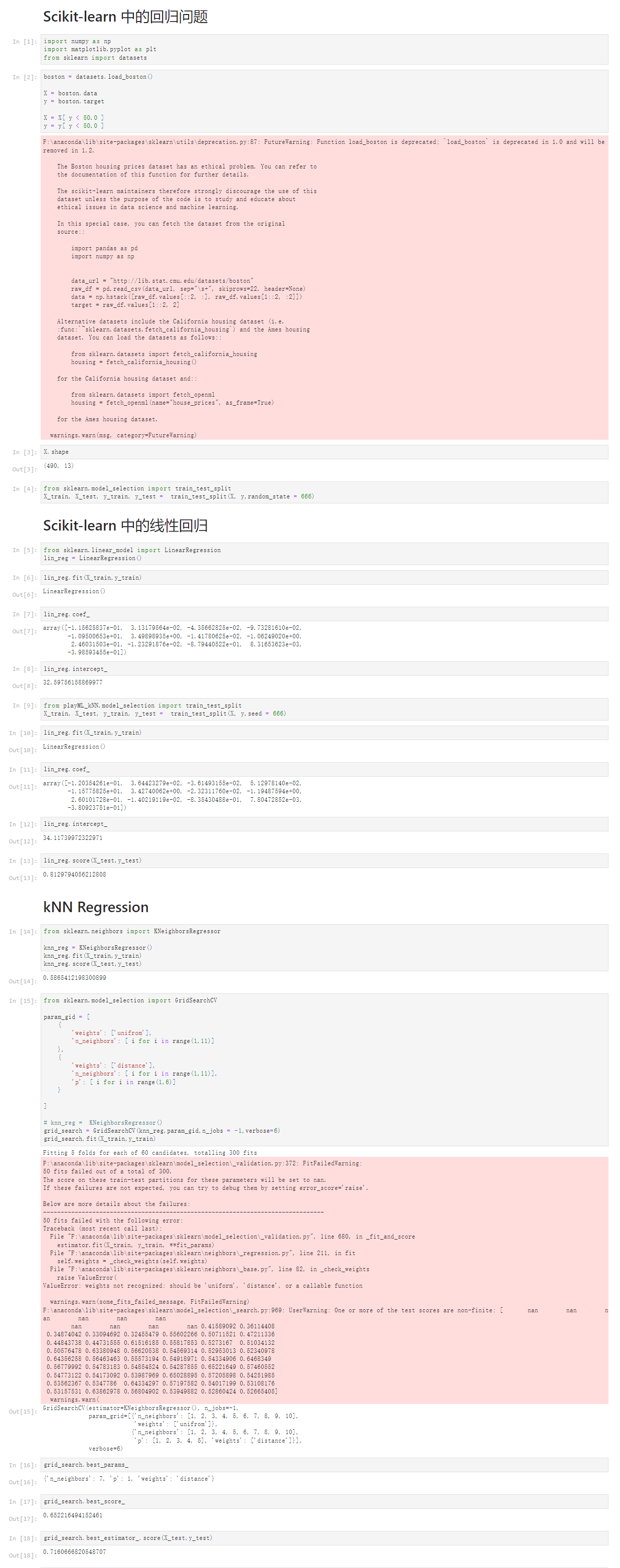
Scikit-learn 中的回归问题
[1]
import numpy as np
import matplotlib.pyplot as plt
from sklearn import datasets
[2]
boston = datasets.load_boston()

X = boston.data
y = boston.target

X = X[ y < 50.0 ]
y = y[ y < 50.0 ]
F:\anaconda\lib\site-packages\sklearn\utils\deprecation.py:87: FutureWarning: Function load_boston is deprecated; `load_boston` is deprecated in 1.0 and will be removed in 1.2.

    The Boston housing prices dataset has an ethical problem. You can refer to
    the documentation of this function for further details.

    The scikit-learn maintainers therefore strongly discourage the use of this
    dataset unless the purpose of the code is to study and educate about
    ethical issues in data science and machine learning.

    In this special case, you can fetch the dataset from the original
    source::

        import pandas as pd
        import numpy as np


        data_url = "http://lib.stat.cmu.edu/datasets/boston"
        raw_df = pd.read_csv(data_url, sep="\s+", skiprows=22, header=None)
        data = np.hstack([raw_df.values[::2, :], raw_df.values[1::2, :2]])
        target = raw_df.values[1::2, 2]

    Alternative datasets include the California housing dataset (i.e.
    :func:`~sklearn.datasets.fetch_california_housing`) and the Ames housing
    dataset. You can load the datasets as follows::

        from sklearn.datasets import fetch_california_housing
        housing = fetch_california_housing()

    for the California housing dataset and::

        from sklearn.datasets import fetch_openml
        housing = fetch_openml(name="house_prices", as_frame=True)

    for the Ames housing dataset.

  warnings.warn(msg, category=FutureWarning)

[3]
X.shape
(490, 13)
[4]
from sklearn.model_selection import train_test_split
X_train, X_test, y_train, y_test =  train_test_split(X, y,random_state = 666)
Scikit-learn 中的线性回归
[5]
from sklearn.linear_model import LinearRegression
lin_reg = LinearRegression()
[6]
lin_reg.fit(X_train,y_train)
LinearRegression()
[7]
lin_reg.coef_
array([-1.15625837e-01,  3.13179564e-02, -4.35662825e-02, -9.73281610e-02,
       -1.09500653e+01,  3.49898935e+00, -1.41780625e-02, -1.06249020e+00,
        2.46031503e-01, -1.23291876e-02, -8.79440522e-01,  8.31653623e-03,
       -3.98593455e-01])
[8]
lin_reg.intercept_
32.59756158869977
[9]
from playML_kNN.model_selection import train_test_split
X_train, X_test, y_train, y_test =  train_test_split(X, y,seed = 666)
[10]
lin_reg.fit(X_train,y_train)
LinearRegression()
[11]
lin_reg.coef_
array([-1.20354261e-01,  3.64423279e-02, -3.61493155e-02,  5.12978140e-02,
       -1.15775825e+01,  3.42740062e+00, -2.32311760e-02, -1.19487594e+00,
        2.60101728e-01, -1.40219119e-02, -8.35430488e-01,  7.80472852e-03,
       -3.80923751e-01])
[12]
lin_reg.intercept_
34.11739972322971
[13]
lin_reg.score(X_test,y_test)
0.8129794056212808
kNN Regression
[14]
from sklearn.neighbors import KNeighborsRegressor

knn_reg = KNeighborsRegressor()
knn_reg.fit(X_train,y_train)
knn_reg.score(X_test,y_test)
0.5865412198300899
[15]
from sklearn.model_selection import GridSearchCV

param_gid = [
    {
        'weights': ['unifrom'],
        'n_neighbors': [ i for i in range(1,11)]
    },
    {
        'weights': ['distance'],
        'n_neighbors': [ i for i in range(1,11)],
        'p': [ i for i in range(1,6)]
    }

]

# knn_reg =  KNeighborsRegressor()
grid_search = GridSearchCV(knn_reg,param_gid,n_jobs = -1,verbose=6)
grid_search.fit(X_train,y_train)

Fitting 5 folds for each of 60 candidates, totalling 300 fits

F:\anaconda\lib\site-packages\sklearn\model_selection\_validation.py:372: FitFailedWarning:
50 fits failed out of a total of 300.
The score on these train-test partitions for these parameters will be set to nan.
If these failures are not expected, you can try to debug them by setting error_score='raise'.

Below are more details about the failures:
--------------------------------------------------------------------------------
50 fits failed with the following error:
Traceback (most recent call last):
  File "F:\anaconda\lib\site-packages\sklearn\model_selection\_validation.py", line 680, in _fit_and_score
    estimator.fit(X_train, y_train, **fit_params)
  File "F:\anaconda\lib\site-packages\sklearn\neighbors\_regression.py", line 211, in fit
    self.weights = _check_weights(self.weights)
  File "F:\anaconda\lib\site-packages\sklearn\neighbors\_base.py", line 82, in _check_weights
    raise ValueError(
ValueError: weights not recognized: should be 'uniform', 'distance', or a callable function

  warnings.warn(some_fits_failed_message, FitFailedWarning)
F:\anaconda\lib\site-packages\sklearn\model_selection\_search.py:969: UserWarning: One or more of the test scores are non-finite: [       nan        nan        nan        nan        nan        nan
        nan        nan        nan        nan 0.41589092 0.36114408
 0.34874042 0.33094692 0.32455479 0.55602266 0.50711521 0.47211336
 0.44843738 0.44731555 0.61516185 0.55817853 0.5273167  0.51034132
 0.50576478 0.63380948 0.56620538 0.54569314 0.52953013 0.52340978
 0.64356258 0.56463463 0.55573194 0.54918971 0.54334906 0.6468349
 0.56779992 0.54783183 0.54854524 0.54287855 0.65221649 0.57460552
 0.54773122 0.54173092 0.53987969 0.65028895 0.57205898 0.54251985
 0.53562367 0.5347786  0.64334297 0.57197582 0.54017199 0.53108176
 0.53157531 0.63862978 0.56804902 0.53949882 0.52860424 0.52665405]
  warnings.warn(

GridSearchCV(estimator=KNeighborsRegressor(), n_jobs=-1,
             param_grid=[{'n_neighbors': [1, 2, 3, 4, 5, 6, 7, 8, 9, 10],
                          'weights': ['unifrom']},
                         {'n_neighbors': [1, 2, 3, 4, 5, 6, 7, 8, 9, 10],
                          'p': [1, 2, 3, 4, 5], 'weights': ['distance']}],
             verbose=6)
[16]
grid_search.best_params_
{'n_neighbors': 7, 'p': 1, 'weights': 'distance'}
[17]
grid_search.best_score_
0.652216494152461
[18]
grid_search.best_estimator_.score(X_test,y_test)
0.7160666820548707
5-10 线性回归的可解性和更多思考


Notbook 示例
Notbook 源码
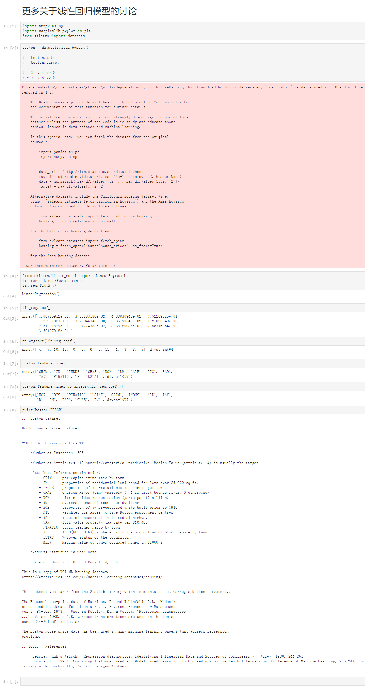
更多关于线性回归模型的讨论
[1]
import numpy as np
import matplotlib.pyplot as plt
from sklearn import datasets
[2]
boston = datasets.load_boston()

X = boston.data
y = boston.target

X = X[ y < 50.0 ]
y = y[ y < 50.0 ]
F:\anaconda\lib\site-packages\sklearn\utils\deprecation.py:87: FutureWarning: Function load_boston is deprecated; `load_boston` is deprecated in 1.0 and will be removed in 1.2.

    The Boston housing prices dataset has an ethical problem. You can refer to
    the documentation of this function for further details.

    The scikit-learn maintainers therefore strongly discourage the use of this
    dataset unless the purpose of the code is to study and educate about
    ethical issues in data science and machine learning.

    In this special case, you can fetch the dataset from the original
    source::

        import pandas as pd
        import numpy as np


        data_url = "http://lib.stat.cmu.edu/datasets/boston"
        raw_df = pd.read_csv(data_url, sep="\s+", skiprows=22, header=None)
        data = np.hstack([raw_df.values[::2, :], raw_df.values[1::2, :2]])
        target = raw_df.values[1::2, 2]

    Alternative datasets include the California housing dataset (i.e.
    :func:`~sklearn.datasets.fetch_california_housing`) and the Ames housing
    dataset. You can load the datasets as follows::

        from sklearn.datasets import fetch_california_housing
        housing = fetch_california_housing()

    for the California housing dataset and::

        from sklearn.datasets import fetch_openml
        housing = fetch_openml(name="house_prices", as_frame=True)

    for the Ames housing dataset.

  warnings.warn(msg, category=FutureWarning)

[4]
from sklearn.linear_model import LinearRegression
lin_reg = LinearRegression()
lin_reg.fit(X,y)
LinearRegression()
[5]
lin_reg.coef_
array([-1.06715912e-01,  3.53133180e-02, -4.38830943e-02,  4.52209315e-01,
       -1.23981083e+01,  3.75945346e+00, -2.36790549e-02, -1.21096549e+00,
        2.51301879e-01, -1.37774382e-02, -8.38180086e-01,  7.85316354e-03,
       -3.50107918e-01])
[6]
np.argsort(lin_reg.coef_)
array([ 4,  7, 10, 12,  0,  2,  6,  9, 11,  1,  8,  3,  5], dtype=int64)
[7]
boston.feature_names
array(['CRIM', 'ZN', 'INDUS', 'CHAS', 'NOX', 'RM', 'AGE', 'DIS', 'RAD',
       'TAX', 'PTRATIO', 'B', 'LSTAT'], dtype='<U7')
[8]
boston.feature_names[np.argsort(lin_reg.coef_)]
array(['NOX', 'DIS', 'PTRATIO', 'LSTAT', 'CRIM', 'INDUS', 'AGE', 'TAX',
       'B', 'ZN', 'RAD', 'CHAS', 'RM'], dtype='<U7')
[9]
print(boston.DESCR)
.. _boston_dataset:

Boston house prices dataset
---------------------------

**Data Set Characteristics:**

    :Number of Instances: 506

    :Number of Attributes: 13 numeric/categorical predictive. Median Value (attribute 14) is usually the target.

    :Attribute Information (in order):
        - CRIM     per capita crime rate by town
        - ZN       proportion of residential land zoned for lots over 25,000 sq.ft.
        - INDUS    proportion of non-retail business acres per town
        - CHAS     Charles River dummy variable (= 1 if tract bounds river; 0 otherwise)
        - NOX      nitric oxides concentration (parts per 10 million)
        - RM       average number of rooms per dwelling
        - AGE      proportion of owner-occupied units built prior to 1940
        - DIS      weighted distances to five Boston employment centres
        - RAD      index of accessibility to radial highways
        - TAX      full-value property-tax rate per $10,000
        - PTRATIO  pupil-teacher ratio by town
        - B        1000(Bk - 0.63)^2 where Bk is the proportion of black people by town
        - LSTAT    % lower status of the population
        - MEDV     Median value of owner-occupied homes in $1000's

    :Missing Attribute Values: None

    :Creator: Harrison, D. and Rubinfeld, D.L.

This is a copy of UCI ML housing dataset.
https://archive.ics.uci.edu/ml/machine-learning-databases/housing/


This dataset was taken from the StatLib library which is maintained at Carnegie Mellon University.

The Boston house-price data of Harrison, D. and Rubinfeld, D.L. 'Hedonic
prices and the demand for clean air', J. Environ. Economics & Management,
vol.5, 81-102, 1978.   Used in Belsley, Kuh & Welsch, 'Regression diagnostics
...', Wiley, 1980.   N.B. Various transformations are used in the table on
pages 244-261 of the latter.

The Boston house-price data has been used in many machine learning papers that address regression
problems.

.. topic:: References

   - Belsley, Kuh & Welsch, 'Regression diagnostics: Identifying Influential Data and Sources of Collinearity', Wiley, 1980. 244-261.
   - Quinlan,R. (1993). Combining Instance-Based and Model-Based Learning. In Proceedings on the Tenth International Conference of Machine Learning, 236-243, University of Massachusetts, Amherst. Morgan Kaufmann.


 405
405


 被折叠的 条评论
为什么被折叠?
被折叠的 条评论
为什么被折叠?
 到【灌水乐园】发言


