


各位童鞋,大家好,又到周一了,今天我们来分享一下一个批次矫正的方法-----liger,在这个之前呢,我分享过Seurat多样本整合去批次的原理,文章在Seurat包其中的FindIntegrationAnchors函数解析,分享了一些去批次的软件,文章在批次效应,单细胞数据用Harmony算法进行批次矫正, 今天我们来分享另外一个批次去除的方法,liger,文章在Single-Cell Multi-omic Integration Compares and Contrasts Features of Brain Cell Identity, 2019年6月发表与cell(顶级期刊了),而同时在另一篇文献中A benchmark of batch-effect correction methods for single-cell RNA sequencing data比较了很多种批次去除批次方法,对Seurat,harmony,liger三种方法的评价最高,但是其中Seurat矫正存在严重的过矫正问题,而harmony目前已经普遍运用,我们今天分享的liger,它的独到之处又是什么呢?为什么可以发到cell,今天我们来参透它,还是原来的方法,先分享文章,后示例代码。
SUMMARY
Defining cell types requires integrating diverse single-cell measurements from multiple experiments and biological contexts(这个不用多介绍了,一个样本发文章的时代早就过去了). To flexibly model singlecell datasets, we developed LIGER, an algorithm that delineates shared and dataset-specific features of cell identity. We applied it to four diverse and challenging analyses of human and mouse brain cells.
(1) First, we defined region-specific and sexually dimorphic gene expression in the mouse bed nucleus of the stria terminalis.(这个地方用到了形态学方法方面的辅助,以检验整合结果的优劣)
(2)Second, we analyzed expression in the human substantia nigra, comparing cell states in specific donors and relating cell types to those in the mouse.(跨物种之间的整合结果检验)
(3)Third, we integrated in situ and singlecell expression data to spatially locate fine subtypes of cells present in the mouse frontal cortex.(原位和单细胞共同的分析检验)。
Finally, we jointly defined mouse cortical cell types using single-cell RNA-seq and DNA methylation profiles(DNA甲基化,这个不是我们今天的重点), revealing putative mechanisms of cell-type-specific epigenomic regulation(表观调控). Integrative analyses using LIGER promise to accelerate investigations of celltype definition, gene regulation, and disease states(让我们拭目以待)。
INTRODUCTION
The function of the mammalian brain is dependent upon the coordinated activity of highly specialized cell types.(第一句话就很重要,强调了细胞空间位置的重要性,这也是为什么现在推出10X空间转录组的原因)。单细胞技术have provided an unprecedented opportunity to systematically identify these cellular specializations,across multiple regions,in the context of perturbations,and in related species(每次读到这里,都会想空间转录组如果也是单细胞精度就非常完美了),Furthermore, new technologies can now measure DNA methylation(甲基化的结果也是非常的重要,大家可以深入的学习,这个方面你的大牛是汤富筹(不知道名字打对了没)),chromatin accessibility(这个就是ATAC),and in situ expression(原位杂交),in thousands to millions of cells.(庞大的单细胞数据目前也是一个大问题,其中张泽民团队研究的新冠文章细胞数量达到恐怖的百万级)Each of these experimental contexts and measurement modalities provides a different glimpse into cellular identity.
Integrative computational tools that can flexibly combine individual single-cell datasets into a unified, shared analysis offer many exciting biological opportunities.(整合分析的必要性),The major challenge of
integrative analysis lies in reconciling the immense heterogeneity observed across individual datasets.(现在不止免疫的个体异质性了,很多都设及到批次)。However, in many kinds of analysis, both dataset similarities and differences are biologically important, such as when we seek to compare and contrast scRNA-seq data from healthy and disease-affected individuals。
To address these challenges, we developed a new computational method called LIGER (linked inference of genomic experimental relationships). We show here that LIGER enables the identification of shared cell types across individuals, species, and multiple modalities (gene expression, epigenetic, or spatial data), as well as dataset-specific features, offering a unified analysis of heterogeneous single-cell datasets.(在这里我们只关注样本的差异去除,至于物种可以了解一下)。
Result1 Comparing and Contrasting Single-Cell Datasets with Shared and Dataset-Specific Factors
LIGER takes as input multiple single-cell datasets, which may be scRNA-seq experiments from different individuals, time points, or species—or measurements from different molecular modalities, such as single-cell epigenome data or spatial gene expression data(个体,物种,技术)

LIGER then employs integrative non-negative matrix factorization (iNMF)(不知道大家对非负矩阵分解有多少了解) to learn a low-dimensional space in which each cell is defined by one set of dataset-specific factors, or metagenes, and another set of shared metagenes。
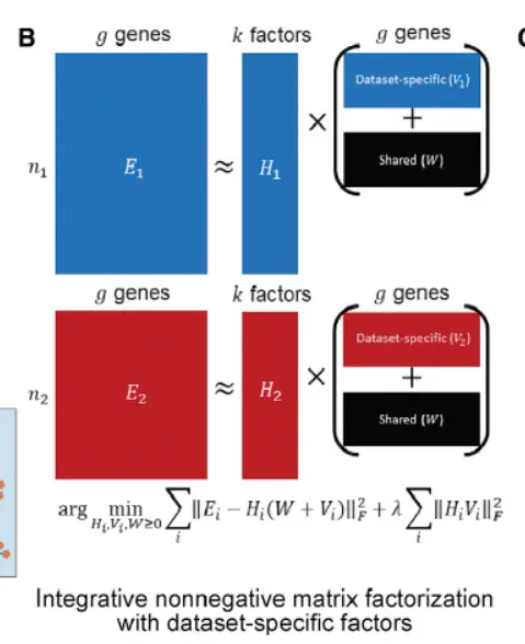
这个图片应该不陌生吧,降维的时候用到的。
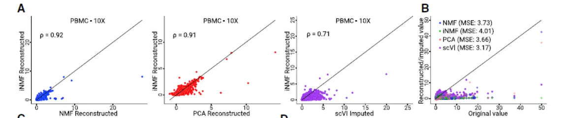
Each factor often corresponds to a biologically interpretable signal—like the genes that define a particular cell type.(不知道大家对降维后每个主成分的研究有多少)。A tuning parameter; λ; allows adjusting the
size of dataset-specific effects to reflect the divergence of the datasets being analyzed. We found that iNMF performs comparably to both NMF and principal-component analysis (PCA) in reconstructing the original data(肯定是差不多的)
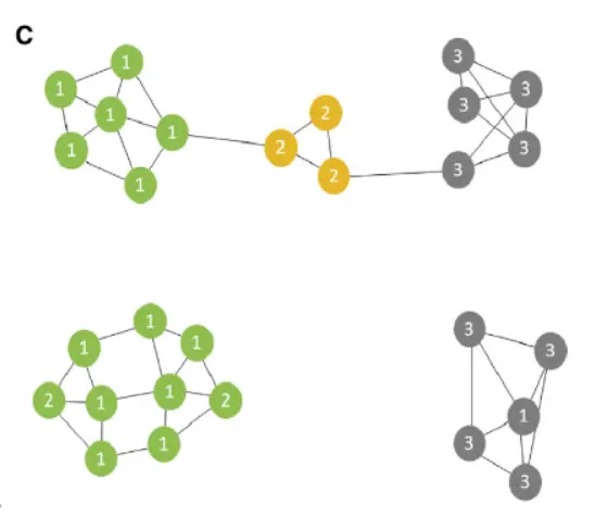
,After performing iNMF, we use a novel strategy that increases robustness of joint clustering.We first assign each cell a label based on themaximum factor loading and then build a shared factor neighborhood graph ,in which we connect cells that have similar factor loading patterns(这个很智慧,需要格外注意)。
We derived a novel algorithm for iNMF optimization, which scales well with the size of large single-cell datasets,To aid selection of the key parameters—the number of factors k and the tuning parameter λ—we developed heuristics based on factor entropy and dataset alignment(看看如何启发的)
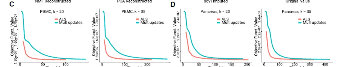
Overall, these heuristics performed well across different analyses ,though we have observed that manual tuning can sometimes improve the results.(下图):
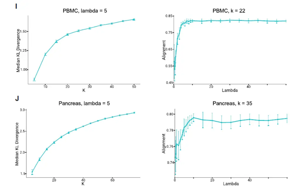
Additionally, we derived novel algorithms for rapidly updating the factorization to incorporate new data or change parameters,We anticipate that this capability will be useful for leveraging a rapidly growing corpus of single-cell data.(其实一但涉及人工调整参数,就需要我们有很强的生物学背景)。
Result2 Liger Shows Robust Performance on Highly Divergent Datasets
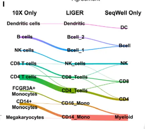
We assessed the performance of LIGER through the use of two metrics: alignment and agreement(这里应该理解为指标)。Alignment measures the uniformity of mixing for two or more samples in the aligned latent space.(衡量对齐的潜在空间中两个或多个样本的混合均匀性。),This metric should be high when datasets share underlying cell types, and low when datasets do not share cognate populations.(我们暂且记住这个注释)。The second metric,agreement, quantifies the similarity of each cell’s neighborhood when a dataset is analyzed separately versus jointly with other datasets(量化相似性)。High agreement indicates that cell-type relationships are preserved with minimal distortion in the joint analysis.(高度aggrement表明,在联合分析中,细胞类型关系得以保留,并且失真最小)。
We calculated alignment and agreement metrics using published datasets,comparing the LIGER analyses to those generated by the Seurat package(和Seurat相比较),We first ran our analyses on a pair of scRNA-seq datasets from human blood cells that show primarily technical differences(技术上带来的批次),and should thus yield a high degree of alignment. Indeed, LIGER and Seurat show similarly high alignment statistics,and LIGER’s joint clusters match the published cluster assignments for the individual datasets
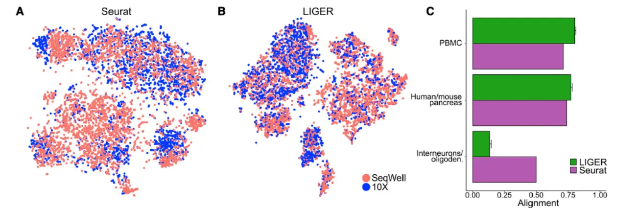
这个地方其实很容易实现,Seurat过矫正,所以对于拥有相同细胞数据类型的整合当然效果很好,而liger采用主成分连接式的方法,当然结果也很不错。
LIGER and Seurat also performed similarly when integrating human and mouse pancreatic data, with LIGER showing slightly higher alignment(跨物种整合,这个不太建议大家做)。
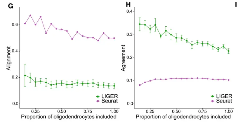
In both analyses, LIGER produced considerably higher agreement than Seurat,suggesting better preservation of the underlying cell-type architectures in the integrated space.We expected this advantage should be especially beneficial when analyzing very divergent datasets that share few or no common cell populations.(这个地方才是我们需要关注的重点,看看结果),LIGER generated minimal false alignment between these classes and demonstrated a good preservation of complex internal substructure(这个时候就要体现数据之间的差异性了)。
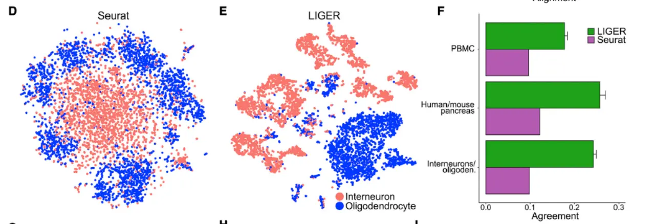
even across considerable changes in dataset proportion,
In each of the three analyses described above, the LIGER joint clustering result closely matched the published cluster assignments for the individual datasets(匹配性很好)。
Together, these analyses indicate that LIGER sensitively detects common populations without spurious alignment and preserves complex substructure, even when applied across divergent datasets(这个地方我们最希望看到的就是不同样本之间的生物学差异)。
Result 3 Interpretable Factors Unravel Complex and Dimorphic Expression Patterns in the Bed Nucleus
An important application of integrative single-cell analysis in neuroscience is to quantify cell-type variation across different brain regions and different members of the same species. To examine LIGER’s performance in these tasks, we analyzed the bed nucleus of the stria terminalis (BNST), a subcortical region composed of multiple subnuclei,implicated in social, stress-related, and reward behaviors,To date, scRNA-seq has not been performed on BNST, providing an opportunity to clarify how cell types are shared between this structure and datasets generated from related tissues.
We isolated, sequenced, and analyzed 204,737 nuclei enriched for the BNST region。Initial clustering identified 106,728 neurons, of which 70.2% were localized to BNST by examination of marker expression in the Allen Brain Atlas (ABA),Clustering analysis revealed 41 transcriptionally distinct populations of BNST-localized neurons(单纯的聚类分析)
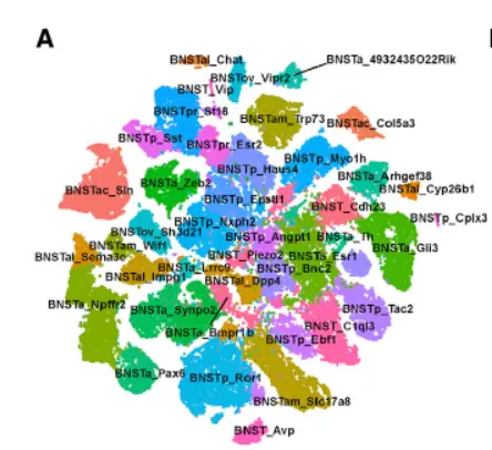
In agreement with previous estimates(跟之前估计的一致),85.9% of the cells were inhibitory
(expressing Gad1 and Gad2), while the remaining 14% were excitatory (expressing Slc17a6 [9.4%] or Slc17a8 [4.7%])
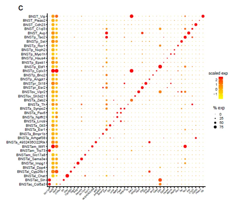
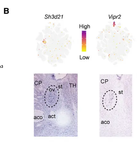
Examination of cluster markers in the ABA showed that many cell types localized to specific BNST substructures, including the principal, oval, and anterior commissure nuclei。For example, we identified two molecularly distinct subpopulations in the oval nucleus of the anterior BNST (ovBNST),a structure known to regulate anxiety and to manifest(显现) a robust circadian rhythm of expression of Per2, similar to the superchiasmatic nucleus (SCN) of the hypothalamus.
Two clusters, BNST_Vip and BNSTp_Cplx3, expressed markers of caudal ganglionic eminence (CGE)-derived interneurons found in cortex and hippocampus. Part of the BNST has embryonic origins in the CGE,suggesting that this structure may harbor such cell types. To examine this possibility, we integrated the 352 nuclei from the BNST_Vip and BNST_Cplx3 clusters with 330 CGE interneuron cell profiles
sampled from our recent adult mouse frontal cortex dataset(我们来看看整合结果), Four clusters in the LIGER analysis showed meaningful alignment between BNST nuclei and cortical CGE cells。
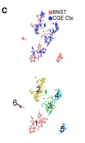
One population (cluster 1), which was Vip-negative and likely localized to the posterior BNST , expressed Id2, Lamp5, Cplx3, and Npy, all markers known to be present in cortical neurogliaform (NG) cells。
A second population (cluster 2) expressed Vip, Htr3a, Cck, and Cnr1, likely corresponding to VIP+ basket cells。
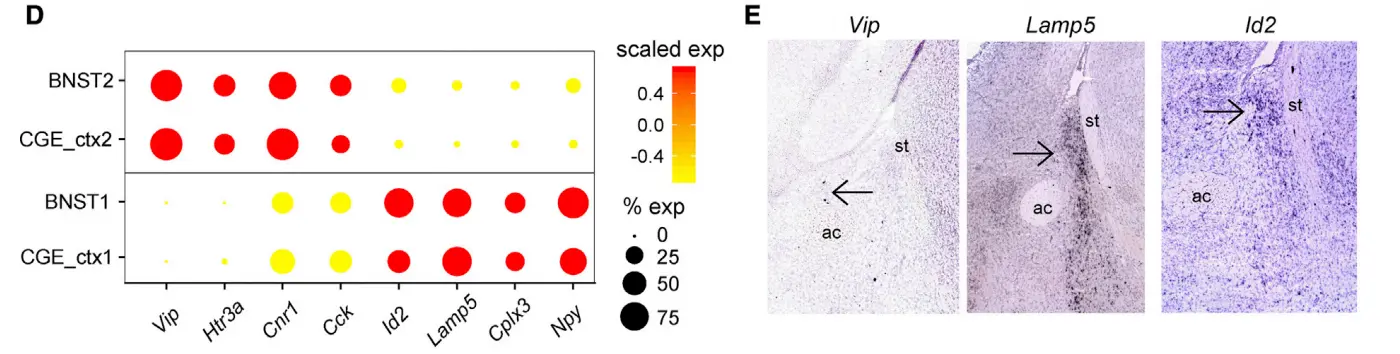
这个地方设及到因子分析,不知道大家没有过多的分析过,我们下一篇文章分享这个,但是这里的差异分析大家要关注一下,不知道大家知不知道这个差异基因排序的原理以及什么软件做的,知道的话,恭喜你,赶紧尝试一下吧。
Result 4 Integration of Substantia Nigra Profiles across Different Human Postmortem Donors and Species
这里对不同技术进行整合,我们简单看一下
我们提炼一下其中的信息:
(1)LIGER accurately integrated each of the cell-type substituents of the SN across datasets
(2)这部分也包括多人和小鼠跨物种的数据整合,总之效果不错。
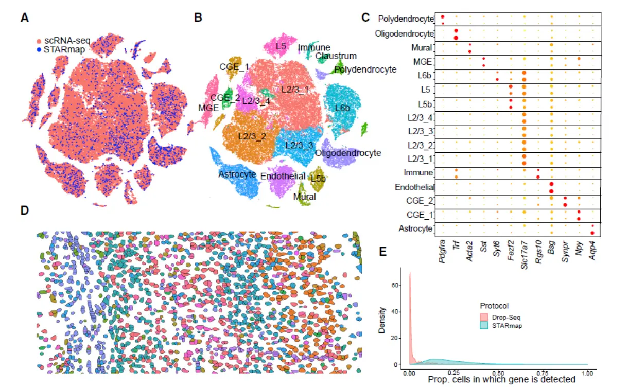
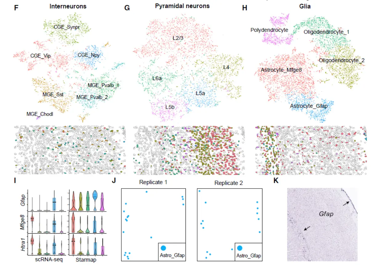
Result5 Integrating scRNA-Seq and In Situ Transcriptomic Data Locates Frontal Cortex Cell Types in Space(这部分结果涉及到空间信息,我们看一下)
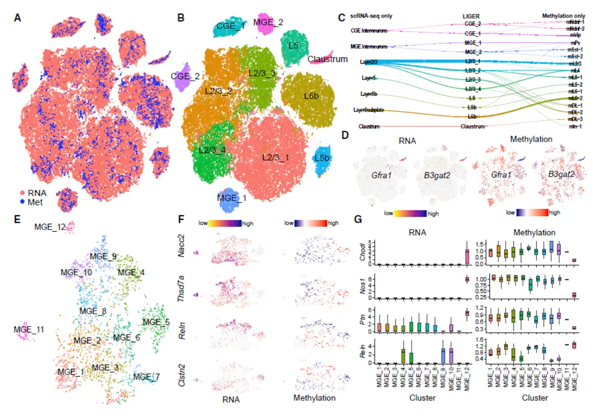
Result 6 LIGER Defines Cell Types Using Both Single-Cell Transcriptome and Single-Cell DNA Methylation Profiles(这部分涉及到甲基化的分析结果,我们简单带过)
Method(我们来看一下其中关键的方法)
(1)Performing iNMF Using Block Coordinate Descent
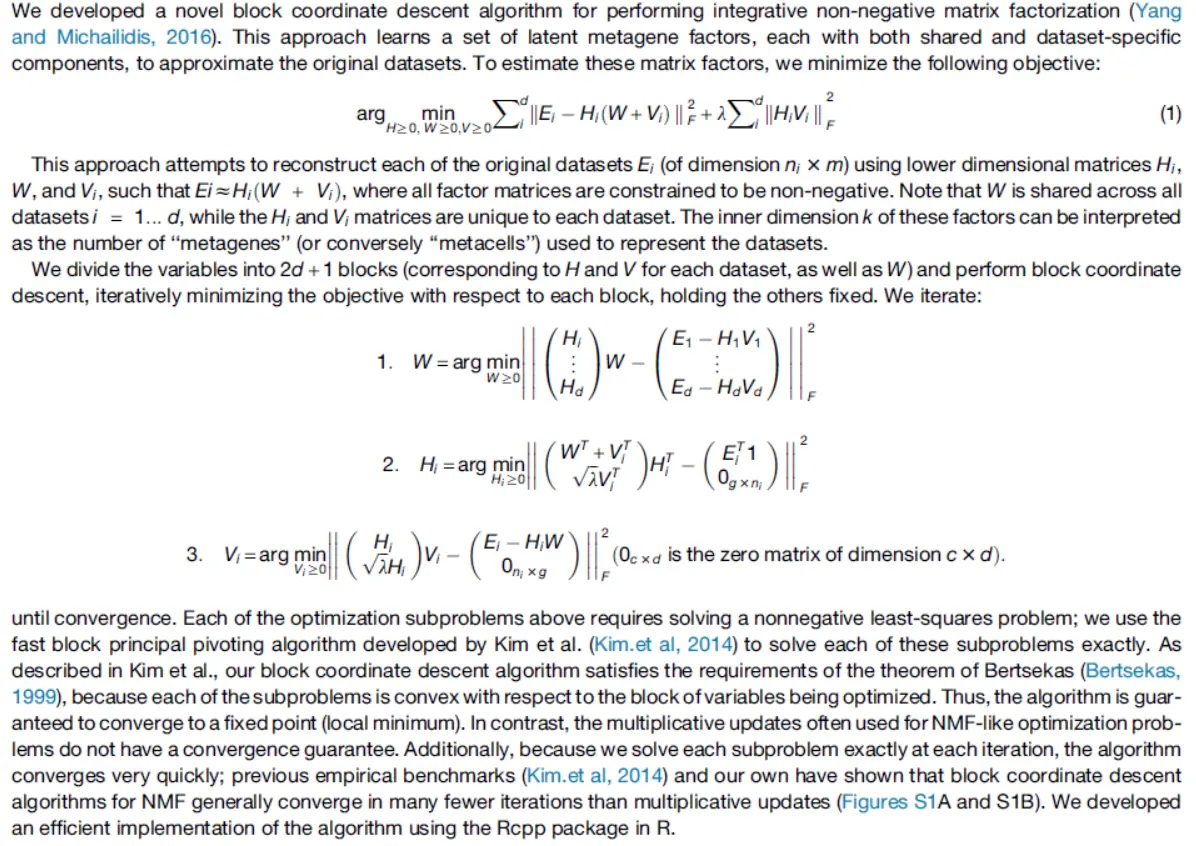
哇,高深的数学让大脑停止运转了。
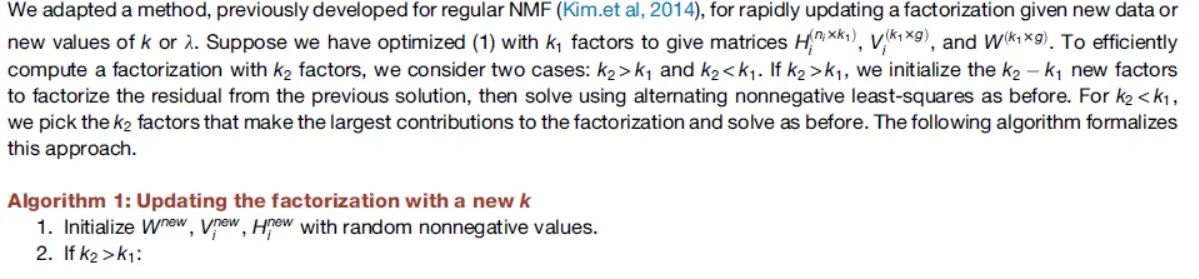
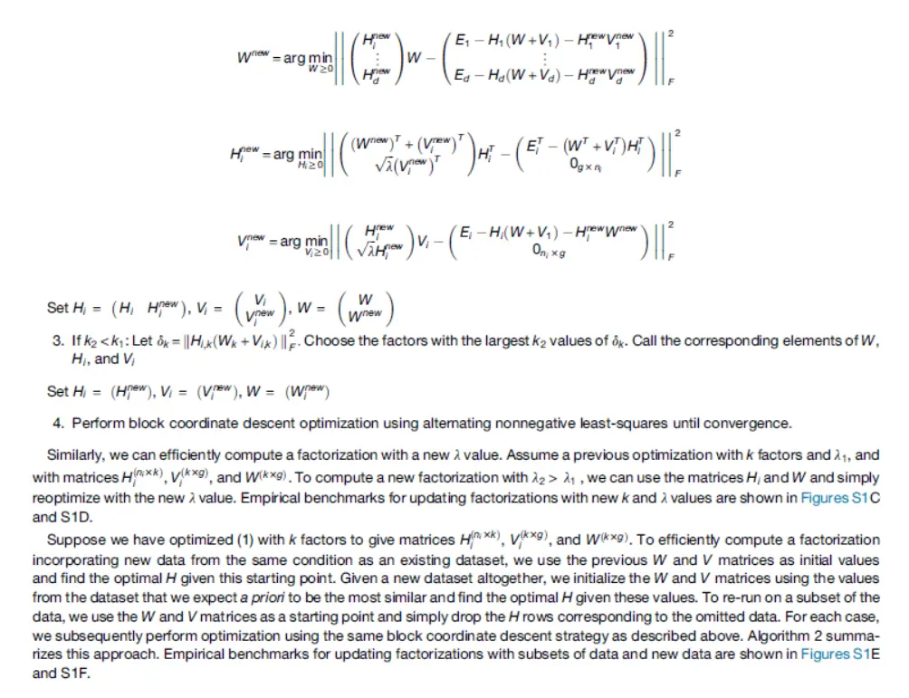
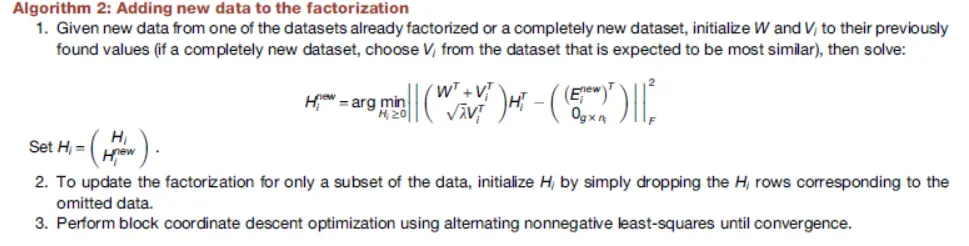
(2)Efficient Updating for New K, New Data, and New λ
(3)Calculating alignment and agreement metrics
最后,我们看一下示例代码
To perform online iNMF, we need to install the latest Liger package from GitHub. Please see the instruction below.
library(devtools)
install_github("welch-lab/liger")
We first create a Liger object by passing the filenames of HDF5 files containing the raw count data. The data can be downloaded here. Liger assumes by default that the HDF5 files are formatted by the 10X CellRanger pipeline. Large datasets are often generated over multiple 10X runs (for example, multiple biological replicates). In such cases it may be necessary to merge the HDF5 files from each run into a single HDF5 file. We provide the mergeH5 function for this purpose (see below for details).
library(rliger)
pbmcs = createLiger(list(stim = "pbmcs_stim.h5", ctrl = "pbmcs_ctrl.h5"))
We then perform the normalization, gene selection, and gene scaling in an online fashion, reading the data from disk in small batches.
pbmcs = normalize(pbmcs)
pbmcs = selectGenes(pbmcs, var.thresh = 0.2, do.plot = F)
pbmcs = scaleNotCenter(pbmcs)
Online Integrative Nonnegative Matrix Factorization
Now we can use online iNMF to factorize the data, again using only minibatches that we read from the HDF5 files on demand (default mini-batch size = 5000). Sufficient number of iterations is crucial for obtaining ideal factorization result. If the size of the mini-batch is set to be close to the size of the whole dataset (i.e. an epoch only contains one iteration), max.epochs needs to be increased accordingly for more iterations.
pbmcs = online_iNMF(pbmcs, k = 20, miniBatch_size = 5000, max.epochs = 5)
Quantile Normalization and Downstream Analysis
After performing the factorization, we can perform quantile normalization to align the datasets.
pbmcs = quantile_norm(pbmcs)
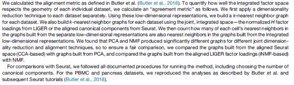
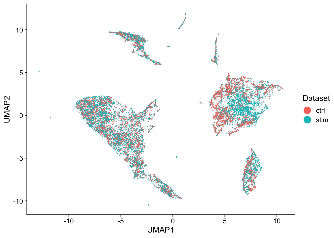
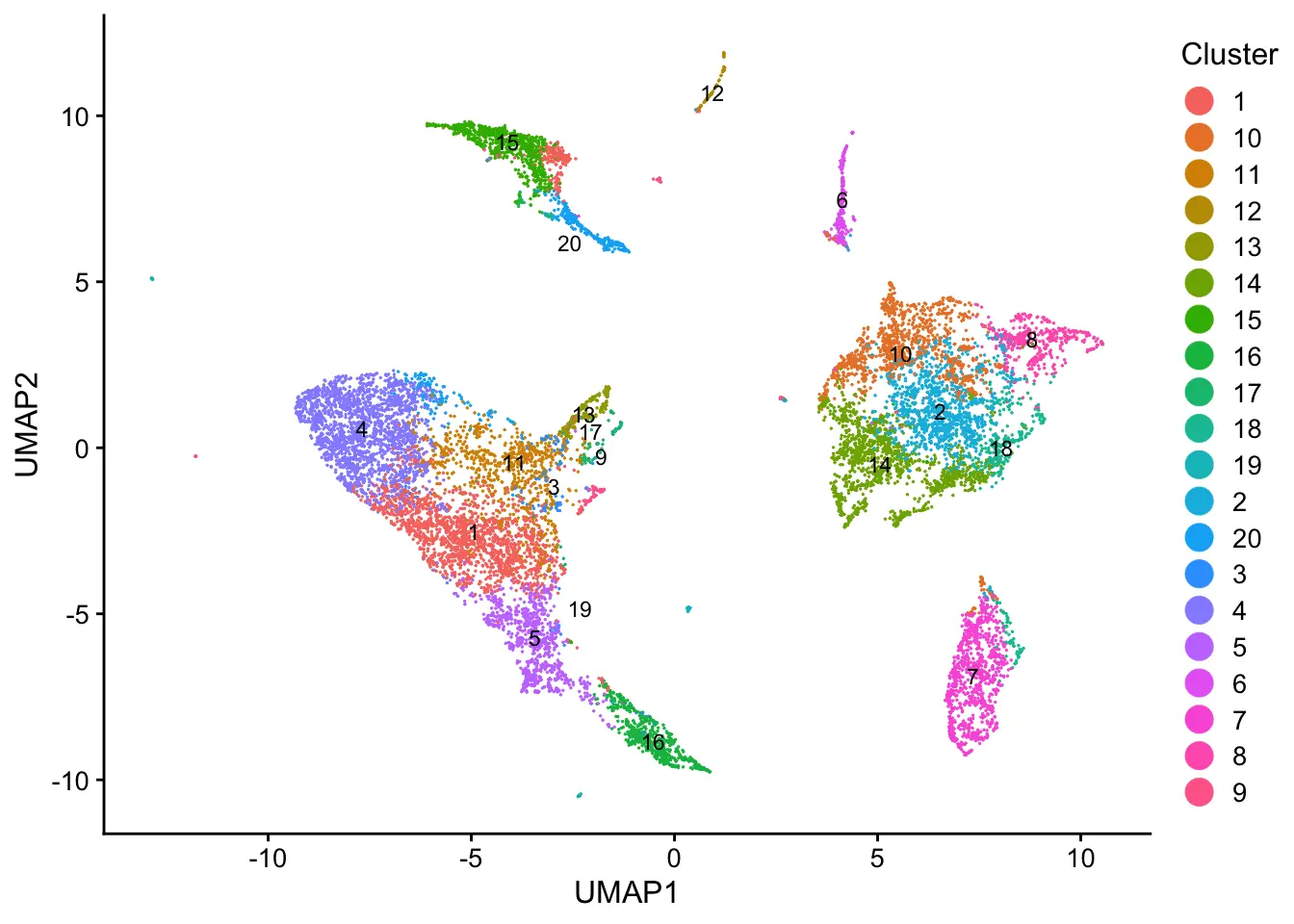
We can also visualize the cell factor loadings in two dimensions using t-SNE or UMAP.
pbmcs = runUMAP(pbmcs)
plotByDatasetAndCluster(pbmcs, axis.labels = c("UMAP1","UMAP2"))
Let’s first evaluate the quality of data alignment. The alignment score ranges from 0 (no alignment) to 1 (perfect alignment).
calcAlignment(pbmcs)
## [1] 0.9149238
With HDF5 files as input, we need to sample the raw, normalized, or scaled data from the full dataset on disk and load them in memory. Some plotting functions and downstream analyses are designed to operate on a subset of cells sampled from the full dataset. This enables rapid analysis using limited memory. The readSubset function allows either uniform random sampling or sampling balanced by cluster. Here we extract the normalized count data of 5000 sampled cells.
pbmcs = readSubset(pbmcs, slot.use = "norm.data", max.cells = 5000)
Using the sampled data stored in memory, we can now compare clusters or datasets (within each cluster) to identify differentially expressed genes. The runWilcoxon function performs differential expression analysis by performing an in-memory Wilcoxon rank-sum test on this subset. Thus, users can still analyze large datasets with a fixed amount of memory.
de_genes = runWilcoxon(pbmcs, compare.method = "datasets")
Here we show the top 10 genes in cluster 1 whose expression level significantly differ between two dataset.
de_genes = de_genes[order(de_genes$padj), ]
head(de_genes[de_genes$group == "1-stim",], n = 10)
##       feature  group    avgExpr     logFC statistic       auc          pval
## 14061   ISG15 1-stim  -5.430433 13.820208  121239.0 0.9898839 6.419043e-114
## 14324    IFI6 1-stim  -6.843238 14.763583  118624.5 0.9685372 2.942152e-108
## 23989   ISG20 1-stim  -5.779989  9.286306  117816.5 0.9619401  4.421875e-99
## 21242   IFIT3 1-stim  -8.320794 14.539736  114625.0 0.9358824  1.133535e-98
## 21244   IFIT1 1-stim  -9.094809 13.669177  112456.0 0.9181731  2.367054e-92
## 27532     MX1 1-stim  -8.935794 12.875135  111536.5 0.9106656  5.884017e-87
## 20364    LY6E 1-stim  -8.721669 12.810795  111435.0 0.9098369  9.506436e-86
## 23754     B2M 1-stim  -3.188800  0.461932  108547.5 0.8862612  3.907049e-69
## 21241   IFIT2 1-stim -11.928663 10.782880  102299.0 0.8352439  3.361002e-66
## 14634  IFI44L 1-stim -12.345872  9.720498   98779.5 0.8065081  3.120570e-55
##                padj pct_in pct_out
## 14061 9.020681e-110    100     100
## 14324 2.067303e-104    100     100
## 23989  2.071354e-95    100     100
## 21242  3.982393e-95    100     100
## 21244  6.652841e-89    100     100
## 27532  1.378135e-83    100     100
## 20364  1.908485e-82    100     100
## 23754  6.863219e-66    100     100
## 21241  5.248019e-63    100     100
## 14634  4.385337e-52    100     100
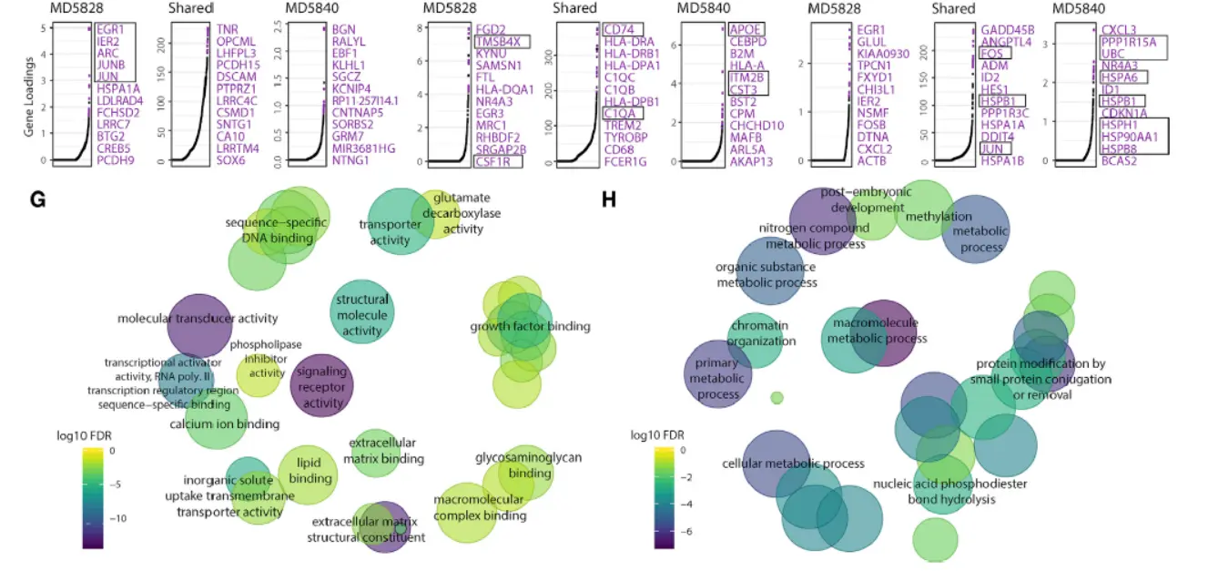
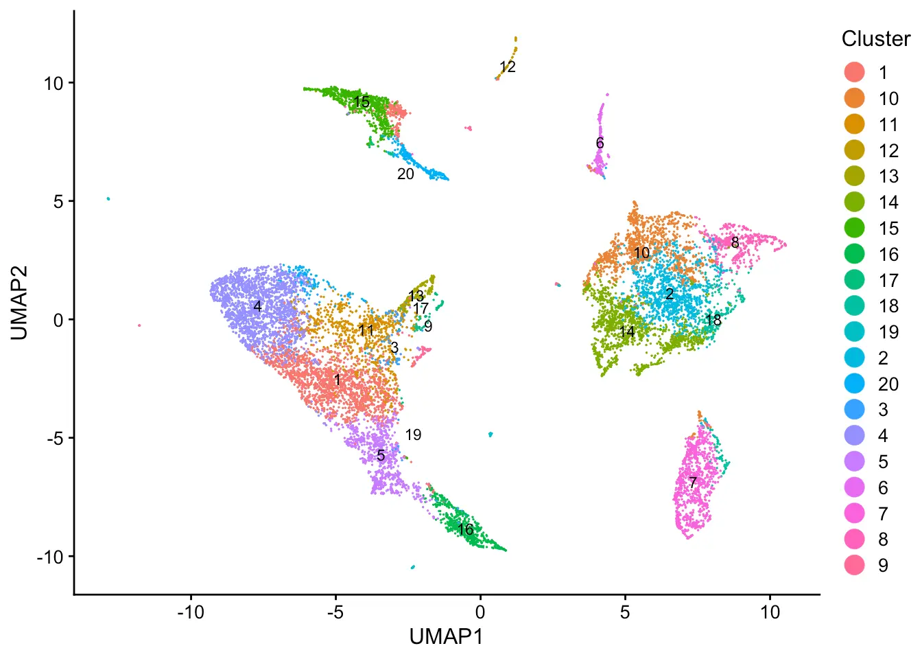
We can show UMAP coordinates of sampled cells by their loadings on each factor (Factor 1 as an example). Underneath it displays the most highly loading shared and dataset-specific genes, with the size of the marker indicating the magnitude of the loading.
p_wordClouds = plotWordClouds(pbmcs, num.genes = 5, return.plots = T)
p_wordClouds[[1]]
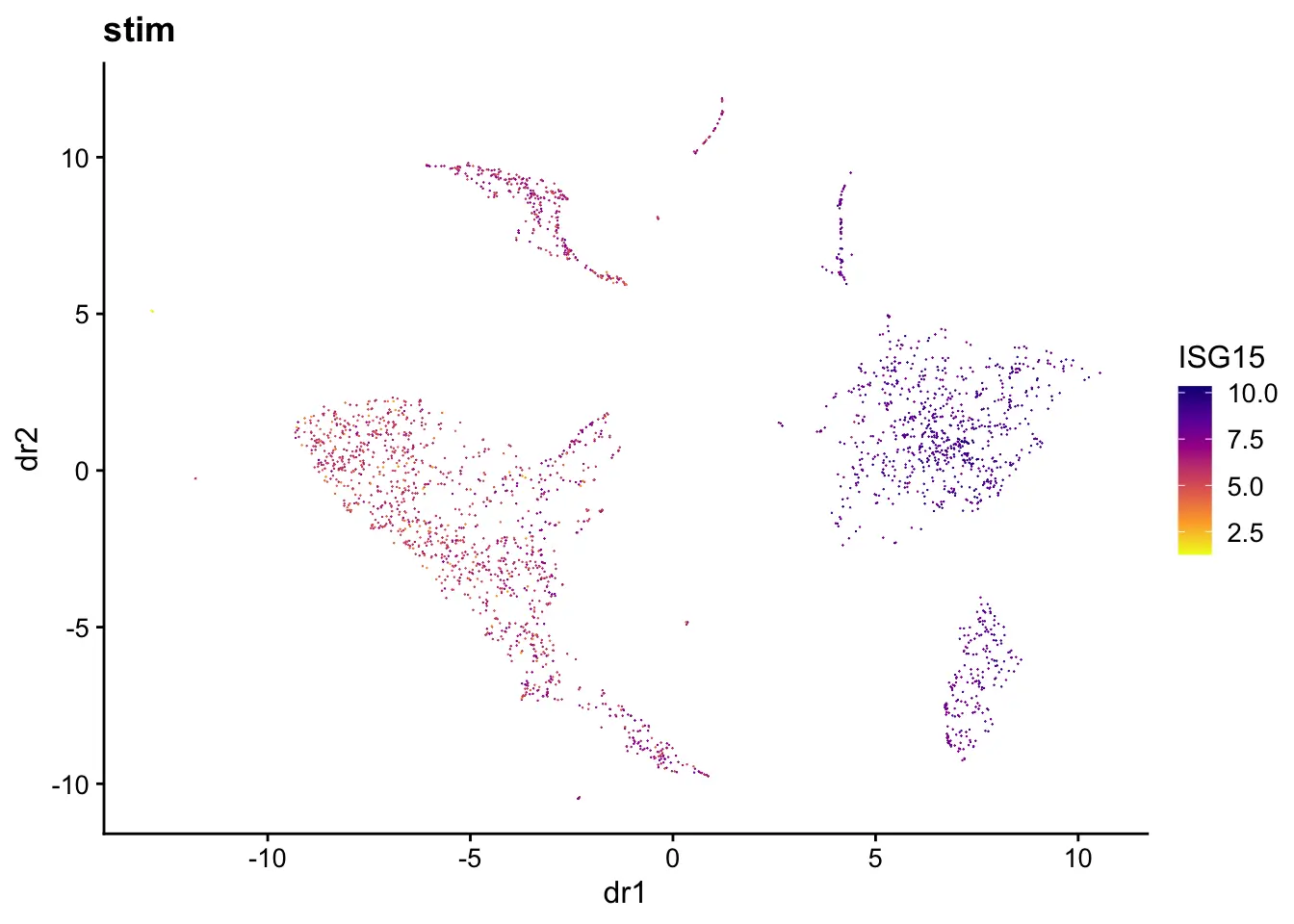
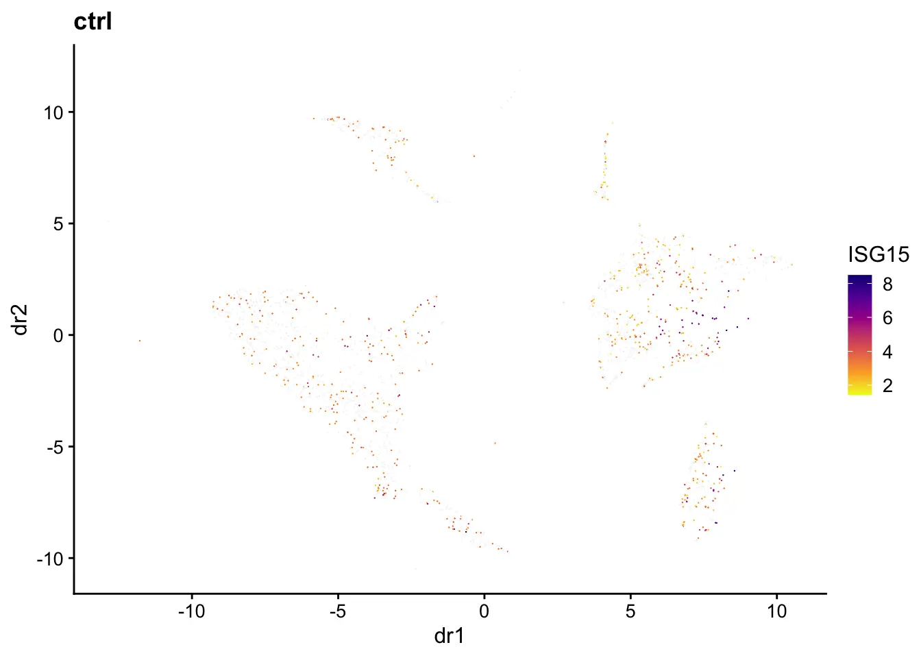
We can generate plots of dimensional reduction coordinates colored by expression of specified gene. The first two UMAP dimensions and gene ISG15 (identified by Wilcoxon test in the previous step) is used as an example here.
plotGene(pbmcs, "ISG15", return.plots = F)
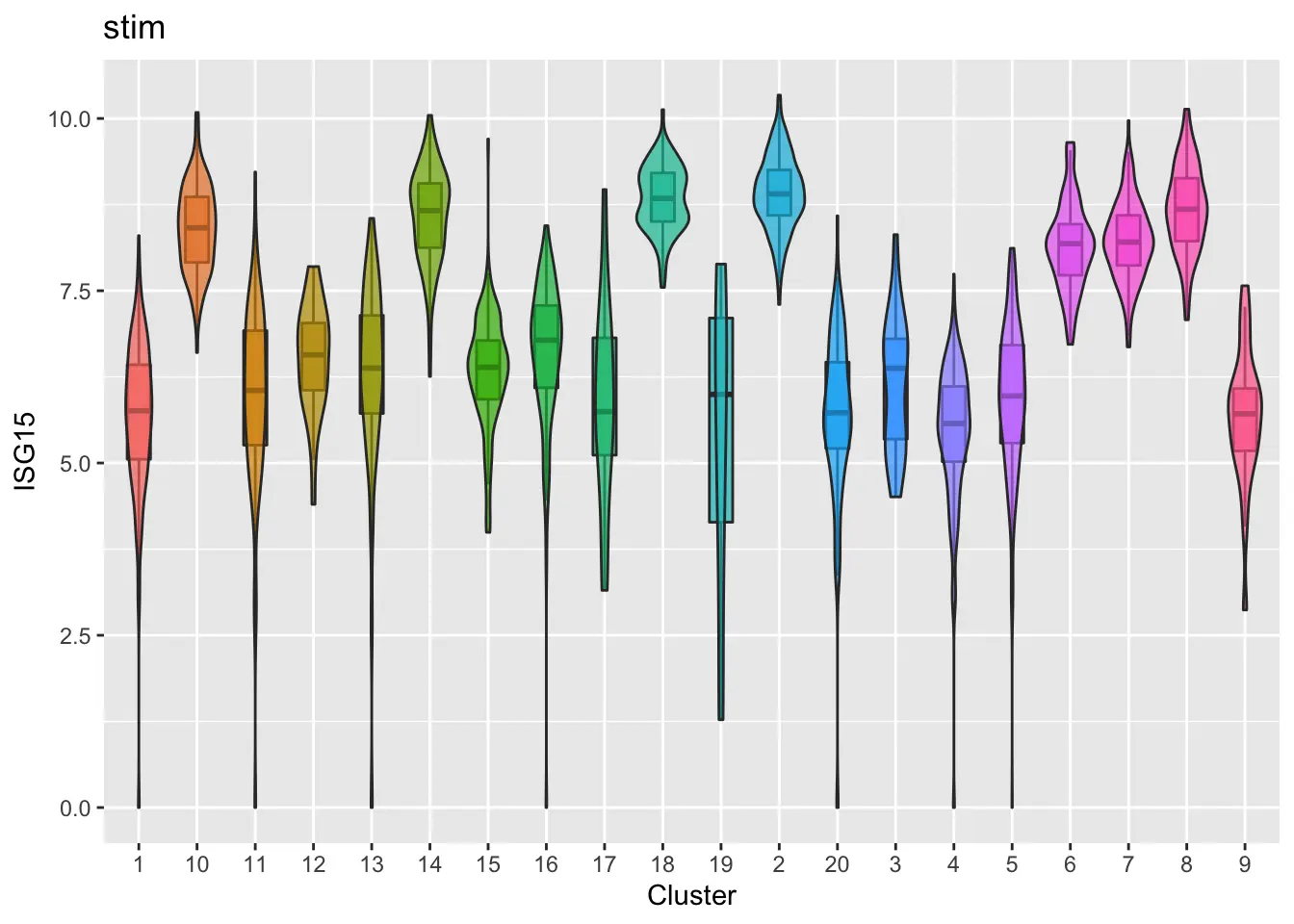
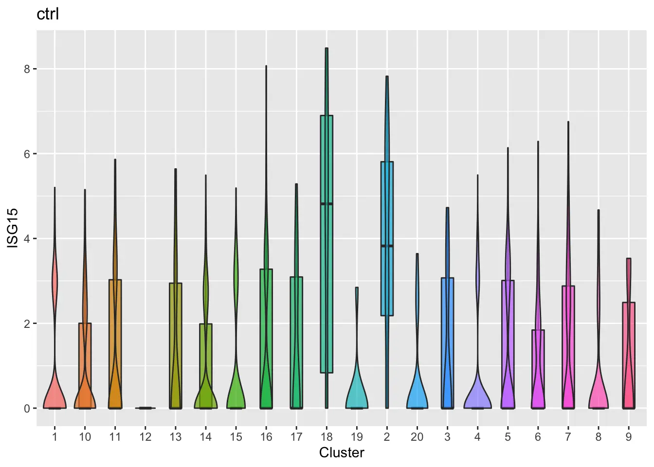
Furthermore, we can make violin plots of expression of specified gene for each dataset (ISG15 as an example).
plotGeneViolin(pbmcs, "ISG15", return.plots = F)
The online algorithm can be implemented on datasets loaded in memory as well. The same analysis is performed on the PBMCs, shown below.
stim = readRDS("pbmcs_stim.RDS")
ctrl = readRDS("pbmcs_ctrl.RDS")
pbmcs_mem = createLiger(list(stim = stim, ctrl = ctrl), remove.missing = F)
pbmcs_mem = normalize(pbmcs_mem)
pbmcs_mem = selectGenes(pbmcs_mem, var.thresh = 0.2, do.plot = F)
pbmcs_mem = scaleNotCenter(pbmcs_mem)
pbmcs_mem = online_iNMF(pbmcs_mem, k = 20, miniBatch_size = 5000, max.epochs = 5)
pbmcs_mem = quantile_norm(pbmcs_mem)
pbmcs_mem = runUMAP(pbmcs_mem)
plotByDatasetAndCluster(pbmcs_mem, axis.labels = c("UMAP1","UMAP2"))

如果有条件的话,不妨试一下,如何灵活运用这个软件,就看大家的需求了
生活很好,有你更好


 被折叠的 条评论
为什么被折叠?
被折叠的 条评论
为什么被折叠?
 到【灌水乐园】发言


