10X空间转录组Visium && HD && Xenium分析全更新

作者，Evil Genius

哎呀， Xenium和HD的空间项目进来了，又要有很多新的工作要做了。

很多分析呢，大家如果只是自己玩一玩，那随便做做就也可以了，但如果像我一样作为公司的分析人员，尤其是大公司的核心分析人员，生信经理之类的，那一定要对自己的分析结果负责，对要求就会高得多,因为分析的水平代表了公司水平。

还有很多人我觉得态度上就有问题，认为官方代码都是现成的，完全不需要公司分析，这种偏见从我做生信就一直有，其实就跟我们上学一样，上高中大家用的一样的教材，都是看的一样的内容，但是高考的结果却是千差万别。cell、nature等高分杂志的文章代码很多都是公开的，但是大家用这些代码能发cell、nature么？再比如单细胞平台，10X单细胞的平台原理大家都知道，但是国内做的水平就是比国外要差，为什么？

其实我们很多都缺乏一种精神，这种精神是在西方世界、包括日本很推崇并且深入骨髓的，那就是工匠精神。

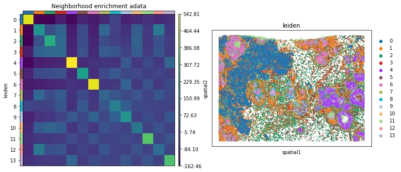
关于Xenium，主推squidpy，文章在高精度空间转录组分析之squidpy和空间网络图,主要分析就是降维聚类和邻域富集分析。

Xenium中，Seurat也出了示例教程，在Analysis of Image-based Spatial Data in Seurat

​

关于HD ，之前分享过STEP，文章在10Xvisium HD高精度平台探索, 主要分析精度为8um 和 16um

​

​

​

​

高精度HD目前Seurat也更新的教程，在Analysis, visualization, and integration of Visium HD spatial datasets with Seurat • Seurat (satijalab.org)

​

总体来讲，python版本的分析更加优秀，这一篇对visium、HD、Xenium

基础分析进行全系列的脚本更新(因为这是公司的要求)。

我们首先来看visium

import CellScopes as cs
sham = cs.read_visium("/home/data/Jia/shamA_visium/MGI0805_A3_147_msham/outs/")

Normalization, dimension reduction and cell clustering

sham = cs.normalize_object(sham; scale_factor = 10000)
sham = cs.scale_object(sham)
sham = cs.find_variable_genes(sham; nFeatures = 1000)
sham = cs.run_pca(sham;  method=:svd, pratio = 1, maxoutdim = 10)
sham = cs.run_umap(sham; min_dist=0.2, n_neighbors=20)
sham = cs.run_clustering(sham; res=0.01, n_neighbors=20)

可视化

cs.dim_plot(sham; dim_type ="umap", marker_size=8)

​

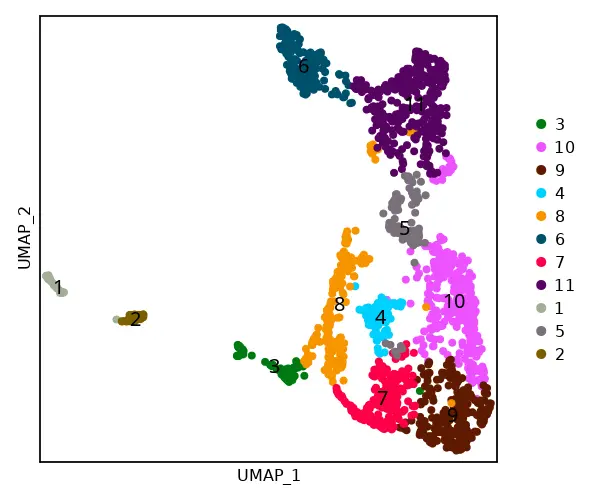
cs.sp_dim_plot(sham, "cluster"; 
    marker_size = 8, width=600, height=500, 
    do_label=false)

​

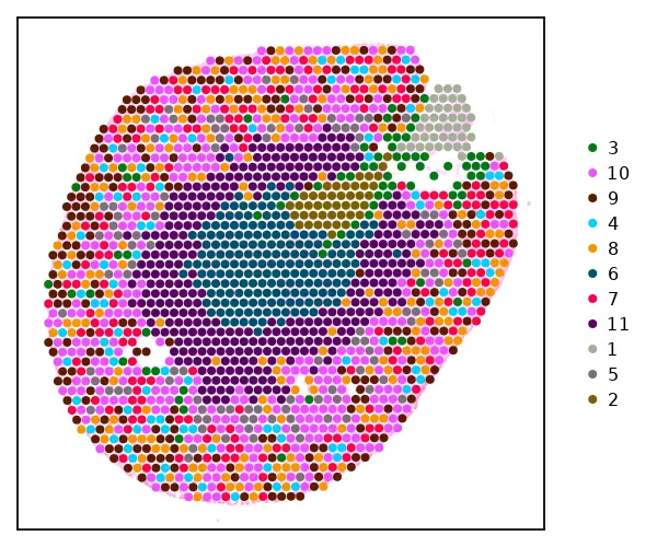
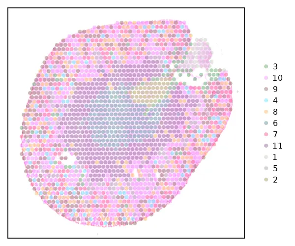
cs.sp_dim_plot(sham, "cluster"; 
    marker_size = 8, width=600, height=500, 
    do_label=false, alpha=0.3)

​

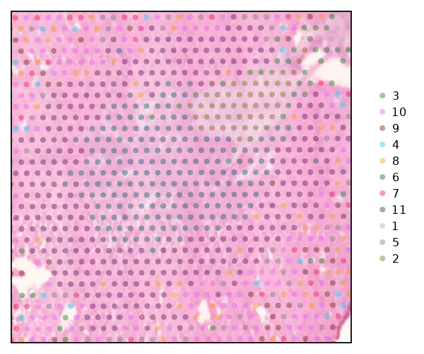
图片剪切

cs.sp_dim_plot(sham, "cluster"; do_label = false, do_legend = true, img_res = "low",
    marker_size = 8, width=600, height=500, adjust_contrast = 1, 
    adjust_brightness= 0.1, alpha =0.4,  x_lims=(200, 440), 
    y_lims=(200, 400))

​

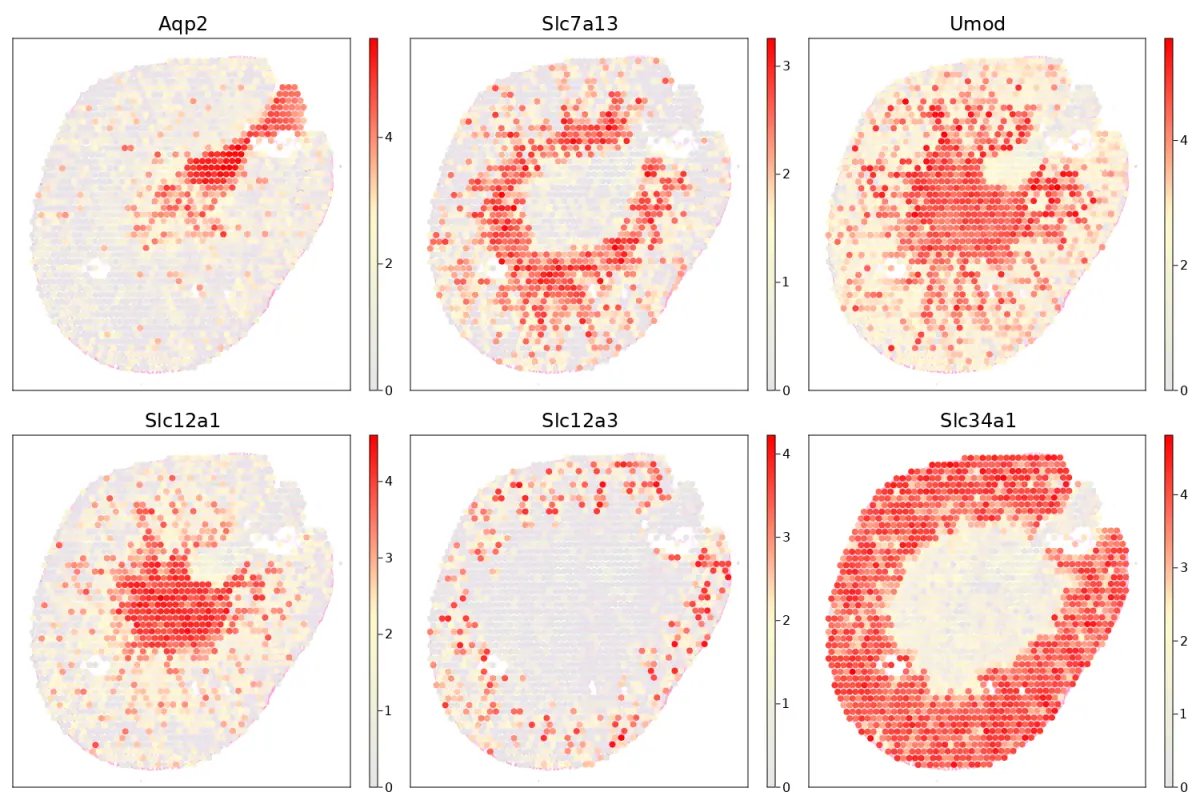
基因可视化

cs.sp_feature_plot(sham, ["Aqp2","Slc7a13", "Umod", "Slc12a1","Slc12a3","Slc34a1"]; 
    marker_size = 8, color_keys=["gray90", "lemonchiffon" ,"red"], 
    adjust_contrast=1, adjust_brightness = 0.3, alpha=1)

​

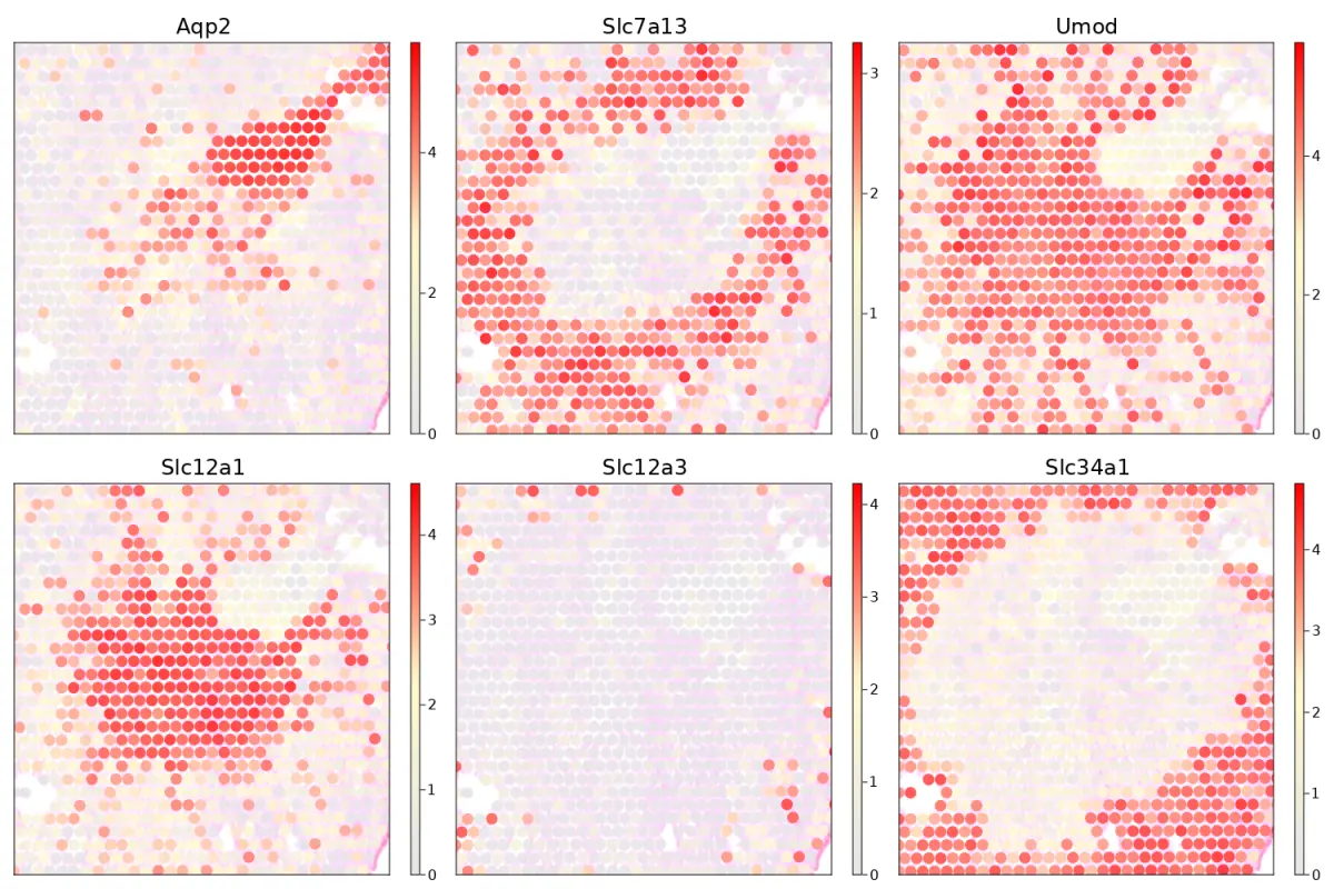
Plot genes on the selected region

cs.sp_feature_plot(sham, ["Aqp2","Slc7a13", "Umod", "Slc12a1","Slc12a3","Slc34a1"]; 
    marker_size = 8, color_keys=["gray90", "lemonchiffon" ,"red"], 
    adjust_contrast=1, adjust_brightness = 0.3, alpha=1,  x_lims=(200, 440), y_lims=(200, 400))

​

接下来我们来看HD，示例数据在 ，其中我们需要注意的是HD可以有多个精度，Data from each bin size is stored in separate layers, which allow users to select data at different resolutions to analyze.，多个精度的分析结果我们都要保留(2um、4um、8um、16um精度)。

import CellScopes as cs
hd_dir = "/mnt/sdb/visiumHD/hd_output/outs/"
hd = cs.read_visiumHD(hd_dir)

1. loading 2um binned data...
Formatting cell polygons...
Progress: 100%[==================================================] Time: 0:00:5039m
1. 2um binned data loaded!
2. loading 8um binned data...
Formatting cell polygons...
Progress: 100%[==================================================] Time: 0:00:08
2. 8um binned data loaded!
3. loading 16um binned data...
Formatting cell polygons...
3. 16um binned data loaded!
VisiumHDObject in CellScopes.jl
Genes x Cells = 18988 x 397258
Available data:
- layerData
- rawCount
- normCount
- scaleCount
- metaData
- spmetaData
- varGene
- dimReduction
- clustData
- imageData
- alterImgData
- polygonData
- defaultData
All fields:
- layerData
- rawCount
- normCount
- scaleCount
- metaData
- spmetaData
- varGene
- dimReduction
- clustData
- imageData
- alterImgData
- polygonData
- defaultData

Layer selection选择，我们需要选择需要分析的精度，当然，也可以是多个精度

hd = cs.set_default_layer(hd; layer_slot = "2_um")
## or
hd = cs.set_default_layer(hd; layer_slot = "16_um")

(Optional) Clustering and dimensional reduction,这一步是可选的，因为Space Ranger已经为8微米和16微米的桶尺寸提供了cluster和UMAP结果。

从8µm bin大小重新聚集细胞可能会很耗时，因为spot数量通常超过300,000。

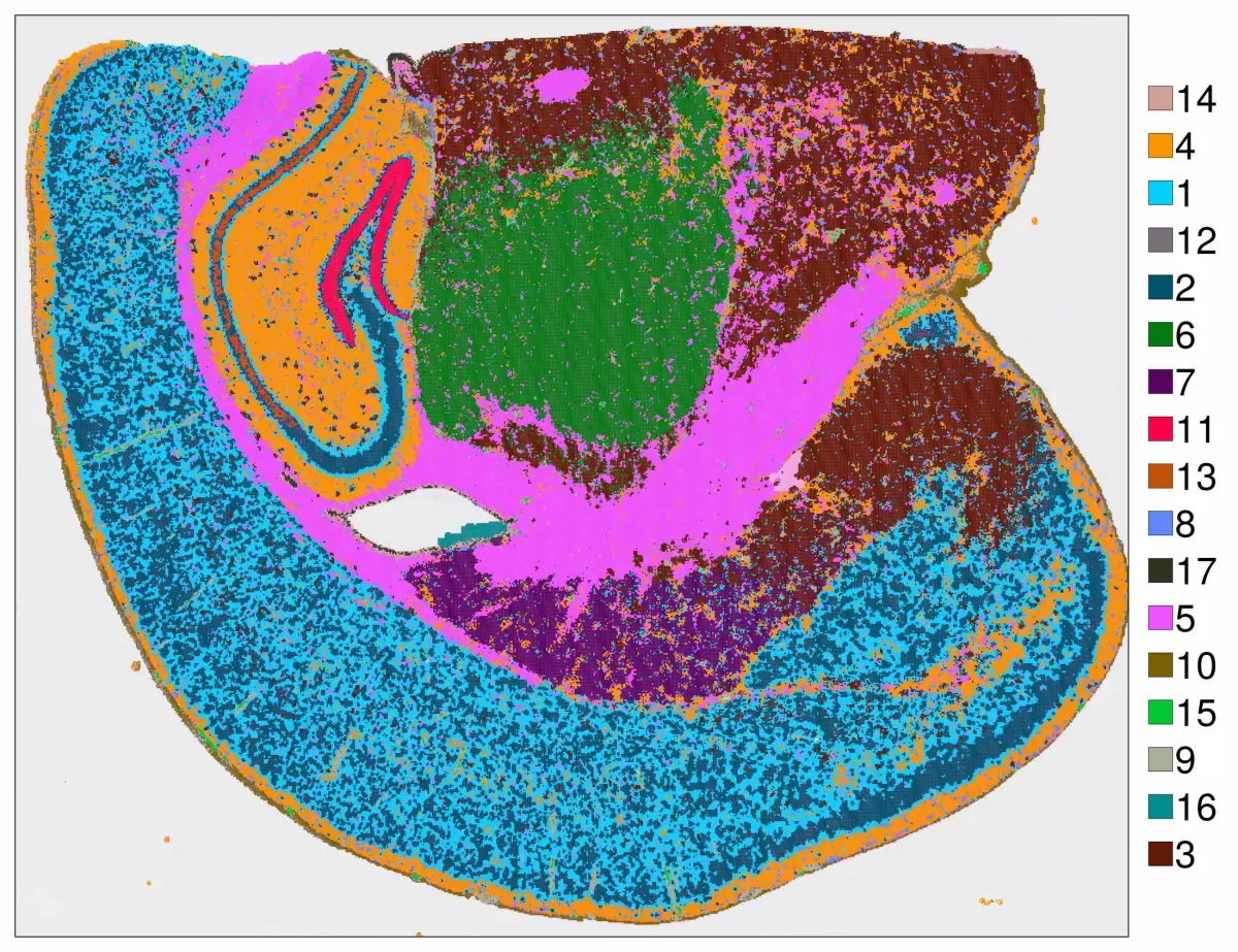
可视化

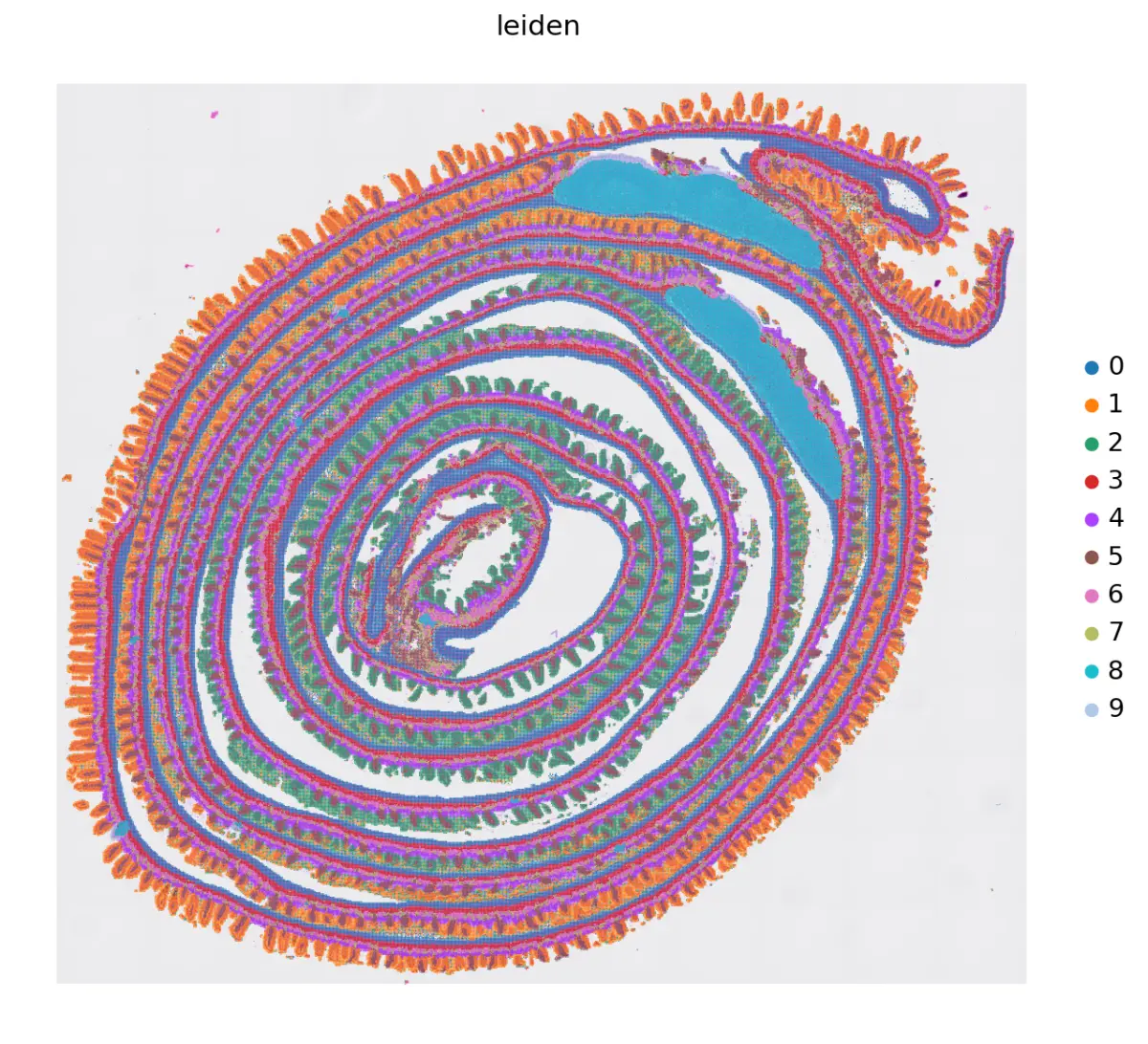
hd = cs.set_default_layer(hd; layer_slot = "8_um")
cs.sp_dim_plot(hd, "cluster"; width=1300, height=1000, 
        do_legend=true, legend_size=40, legend_fontsize=40)

​

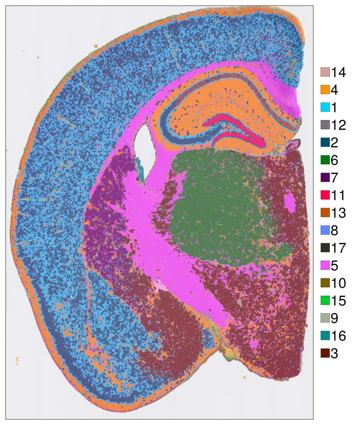
要使方向与原始组织方向对齐，可以使用convert_image_data函数。下面是调整方向的方法:

@time hd = cs.convert_image_data(hd)

转换图像数据后，所有图形将使用调整后的坐标进行可视化。

hd = cs.set_default_layer(hd; layer_slot = "8_um")
cs.sp_dim_plot(hd, "cluster"; width=1300, height=1000, 
        do_legend=true, legend_size=40, legend_fontsize=40)

​

还可以在同一图上突出一个特定的cluster

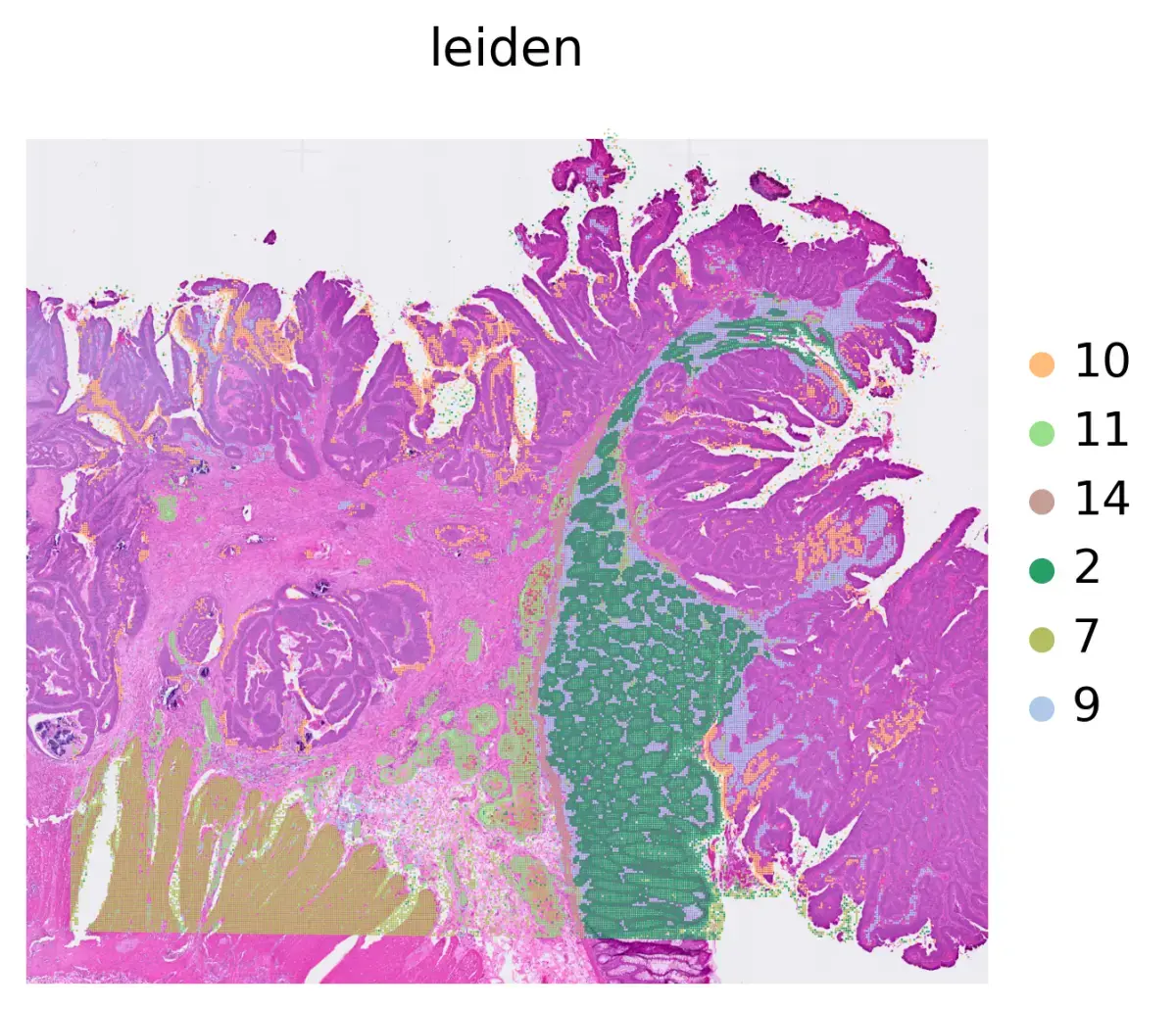
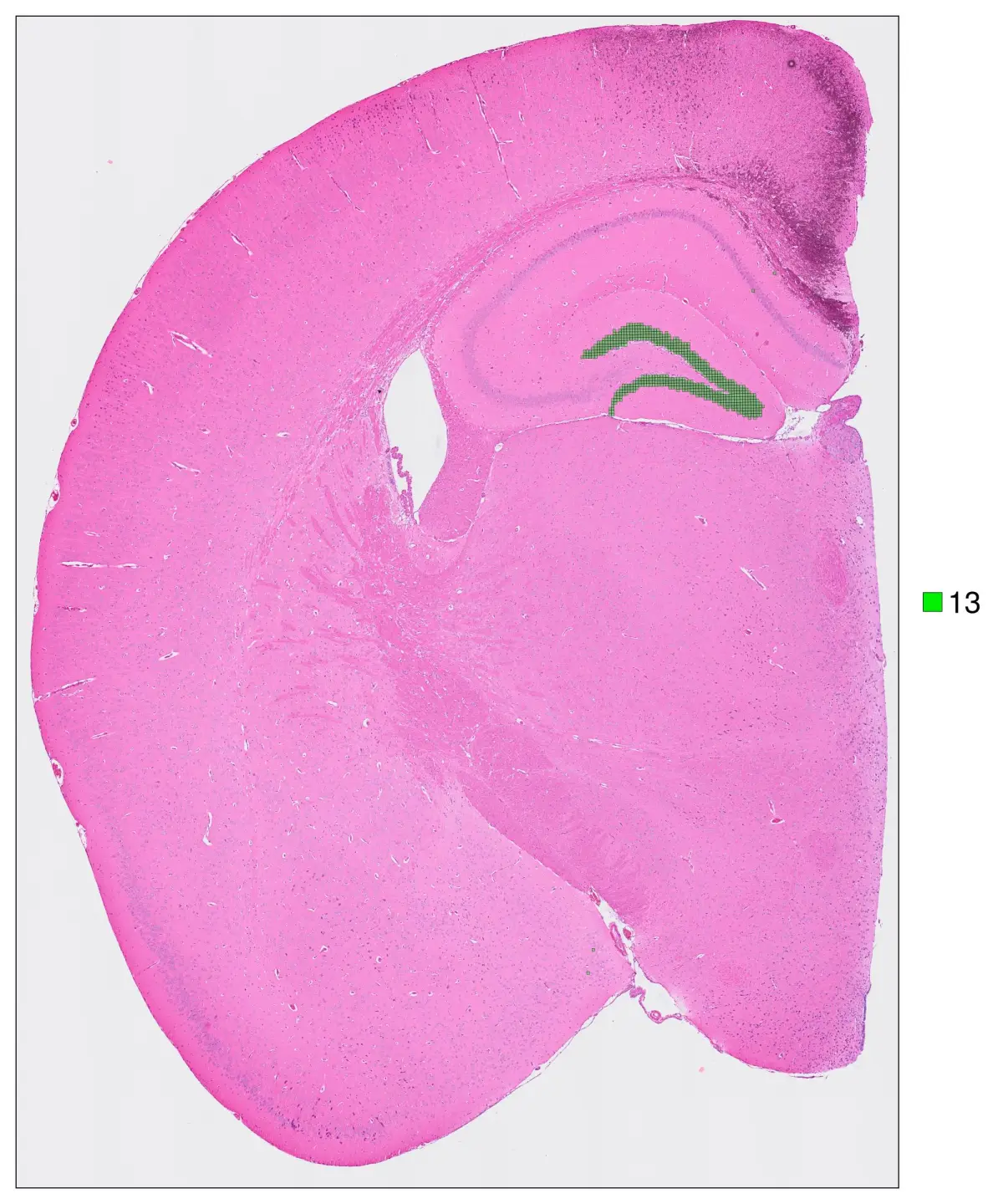
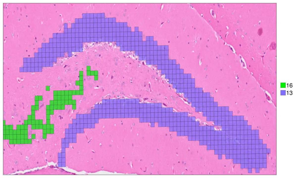
hd = cs.set_default_layer(hd; layer_slot = "16_um")
hd = cs.convert_image_data(hd; layer_slot = "16_um")
cs.sp_dim_plot(hd, "cluster"; width=1000, height=1200, 
          anno_color = Dict("13" => "green2") ,do_legend=true, img_res = "high", stroke_width=0.2, 
            cell_highlight = "13",legend_size=30, adjust_contrast =1, adjust_brightness=0.0, alpha=0.4)

​

Select a region of interest for detailed visualization

cs.plot_fov(hd, 20, 20; marker_size = 0, width=2000, height=2400)

​

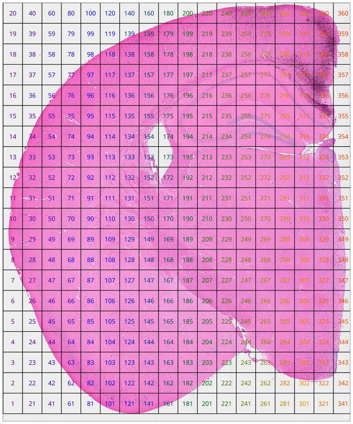
df = cs.subset_fov(hd, [193,197,333,337], 20,20);
xlim, ylim = cs.get_subset_cood(df)
#((9518.974171506527, 17960.0047340106), (14384.796062010153, 20199.649061752563))
####这种初始裁剪可能不会精确地与所需的区域对齐。根据获得的坐标，您可以稍微调整限制以更好地适合您打算关注的区域:
xlim = (9418, 17960)
ylim=(15500, 19799)
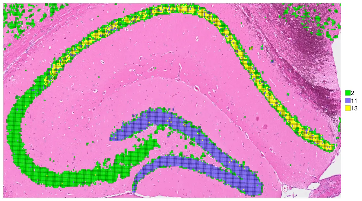
####This method allows you to fine-tune the coordinates manually for an optimal close-up view of your region of interest.
cs.sp_dim_plot(hd, "cluster"; width=1800, height=1000, y_lims=ylim , x_lims=xlim, 
          do_legend=true, img_res = "high", stroke_width=0.4, 
            anno_color = Dict("11" => "slateblue1", "2"=>"green2","13"=>"yellow1"),
            cell_highlight =["11", "2","13"],legend_size=40, 
        adjust_contrast =1, adjust_brightness=0.0, alpha=1)

​

Compare the spatial resolution of different bin sizes

xlim = (11818, 16100)
ylim=(15500, 17599)
hd = cs.set_default_layer(hd; layer_slot = "8_um")
cs.sp_dim_plot(hd, "cluster"; width=1500, height=900, y_lims=ylim , x_lims=xlim, 
          do_legend=true, img_res = "high", stroke_width=0.4, 
            anno_color = Dict("11" => "slateblue1", "2"=>"green2"),
            cell_highlight =["11", "2"],legend_size=40, 
        adjust_contrast =1, adjust_brightness=0.0, alpha=0.7)

​

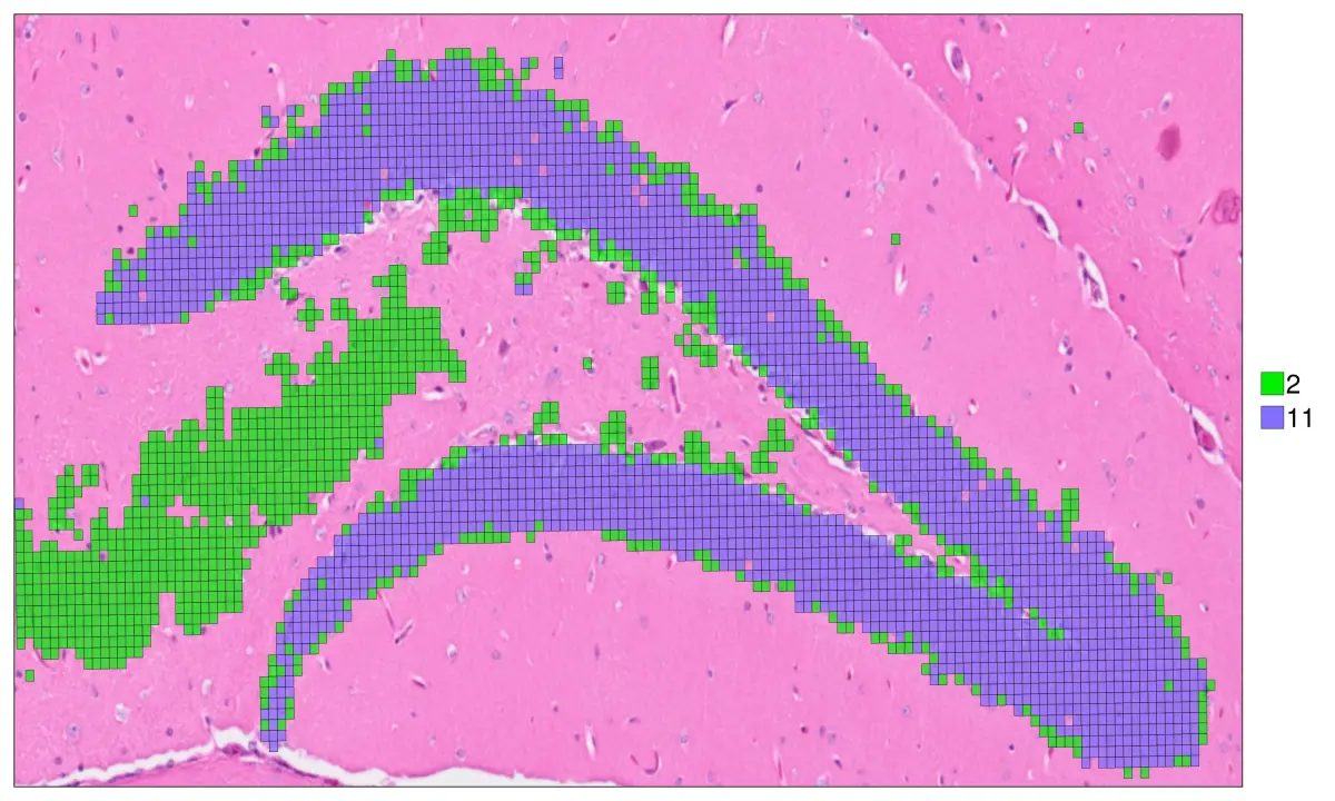
hd = cs.set_default_layer(hd; layer_slot = "16_um")
cs.sp_dim_plot(hd, "cluster"; width=1500, height=900, y_lims=ylim , x_lims=xlim, 
          do_legend=true, img_res = "high", stroke_width=0.4, 
            anno_color = Dict("13" => "slateblue1", "16"=>"green2"),
            cell_highlight =["13", "16"],legend_size=40, 
        adjust_contrast =1, adjust_brightness=0.0, alpha=0.7)

​

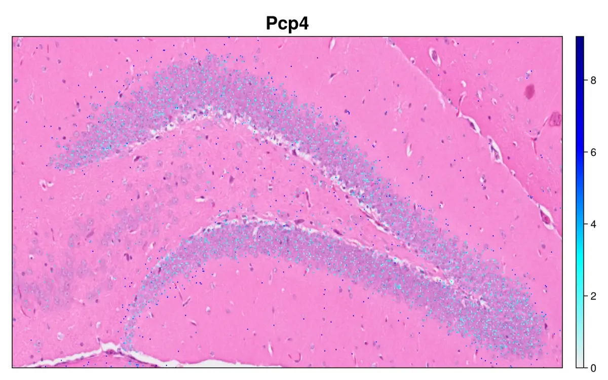
使用sp_feature_plot在不同分辨率下可视化基因表达。

xlim = (11818, 16100)
ylim=(15500, 17599)
hd = cs.set_default_layer(hd; layer_slot="2_um")
hd = cs.normalize_object(hd; scale_factor = 10000)
hd = cs.convert_image_data(hd; layer_slot = "2_um")
cs.sp_feature_plot(hd, ["Pcp4"]; color_keys=["gray94", "cyan", "blue", "darkblue"],  
    width=800, height=500, x_lims=xlim , y_lims=ylim, img_res = "high", alpha=1)

​

hd = cs.set_default_layer(hd; layer_slot="8_um")
hd = cs.normalize_object(hd; scale_factor = 10000)
cs.sp_feature_plot(hd, ["Pcp4"]; color_keys=["gray94", "cyan", "blue", "darkblue"],  
    width=800, height=500, x_lims=xlim , y_lims=ylim, img_res = "high", alpha=1)

​

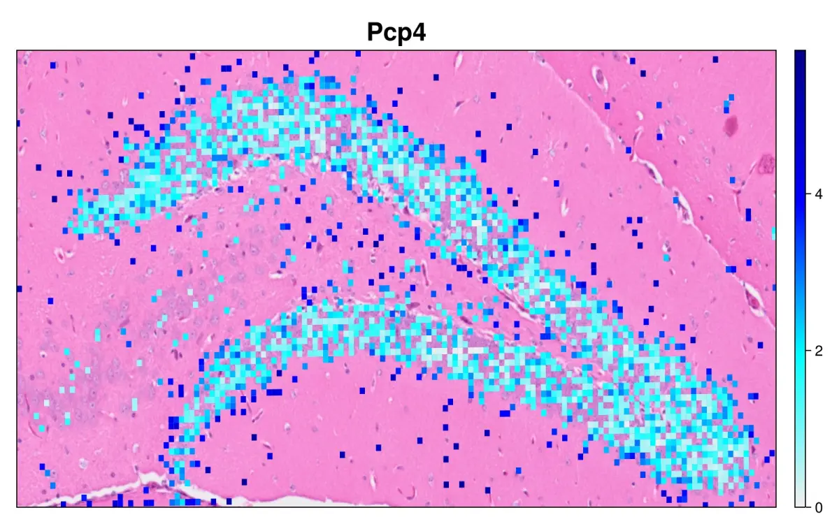
hd = cs.set_default_layer(hd; layer_slot="16_um")
hd = cs.normalize_object(hd; scale_factor = 10000)
cs.sp_feature_plot(hd, ["Pcp4"]; color_keys=["gray94", "cyan", "blue", "darkblue"],  
    width=800, height=500, x_lims=xlim , y_lims=ylim, img_res = "high", alpha=1)

​

写出数据

cs.save(hd; filename="visiumHD.jld2")

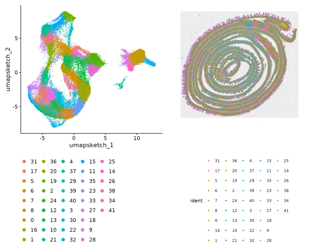
最后来看Xenium

import CellScopes as cs
xenium_dir = "/mnt/sdc/new_analysis_cellscopes/xenium_mouse_brain/"
@time brain = cs.read_xenium(xenium_dir; min_gene = 0, min_cell = 0, prefix = "brain")

Normalization, dimension reduction and cell clustering

brain = cs.normalize_object(brain)
brain = cs.scale_object(brain)
brain = cs.find_variable_genes(brain; nFeatures=200)
brain = cs.run_pca(brain;  method=:svd, pratio = 1, maxoutdim = 20)

(可选)使用Baysor生成细胞多边形，并将基因表达分配给多边形(细胞分割)

Xenium对象已经包含由10x Analyzer生成的细胞多边形数据。如果您想使用其他工具(如Baysor)绘制细胞多边形，请按照以下步骤操作。在生成细胞多边形后，通过运行polygons_cell_mapping将每个多边形与最近的细胞基于欧几里得距离关联起来。最后，需要使用generate_polygon_counts将基因表达值分配给细胞多边形。这一步完全是可选的，可以省略而不影响任何后续的分析。

import Baysor as B
scale=20
min_pixels_per_cell = 15
grid_step = scale / min_pixels_per_cell
bandwidth= scale / 10
count_molecules = deepcopy(brain.spmetaData.molecule)
count_molecules.cell[count_molecules.cell.==-1] .= 0
count_molecules.cell = string.(count_molecules.cell)
cell_baysor = [replace(x, "brain_" => "") for x in count_molecules.cell]
cell_baysor = parse.(Int64, cell_baysor)
polygons = B.boundary_polygons(count_molecules, cell_baysor, grid_step=grid_step, bandwidth=bandwidth)
brain.polygonData = polygons
brain = cs.polygons_cell_mapping(brain)
brain = cs.generate_polygon_counts(brain)

可视化

可视化细胞和基因在降维空间和空间空间上的表达。

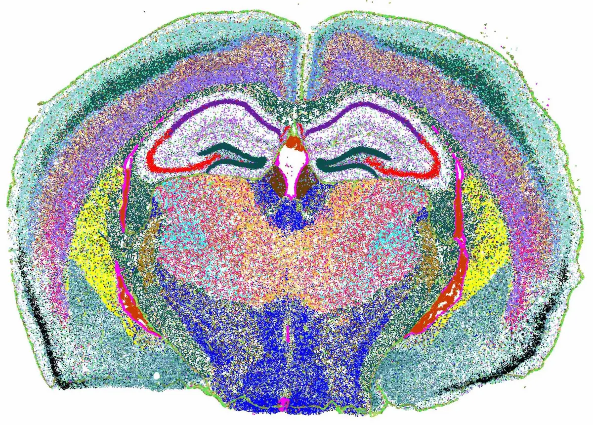
可视化细胞注释

colors =["#4f8c9d", "#8dd2d8", "#0a4f4e", "yellow", "#229743", 
    "#8dd2d8", "#0a4f4e","#a7d64e", "#788c3b", "#57e24c", 
    "#683c00", "#f1bb99", "blue", "#9f1845", 
    "#f87197", "#ff0087", "#a57a6a", "#fabd2a", 
    "#374475", "#628df2", "#691b9e", "slateblue1", 
    "#d5d0fa", "black", "#ab7b05","#4f8c9d",
    "#8dd2d8", "#0a4f4e", "#4aeeb6", "#229743",
    "#a7d64e", "#788c3b", "#57e24c", "#683c00", 
    "#f1bb99", "#db3c18", "cyan", "#f87197", 
    "#ff0087", "#a57a6a", "#fabd2a", "#374475", 
    "#628df2", "#691b9e", "#b25aed", "red", 
    "fuchsia", "#ab7b05","orangered3", "#0a4f4e"]
celltypes = string.(unique(brain.metaData.cluster))
anno_color=Dict(celltypes .=> colors)
cs.sp_dim_plot(brain, "cluster"; anno_color = anno_color,
    do_label = false,marker_size = 5, 
    width=2500, height=2000, do_legend=false
    )

​

Select a field of view to visualize the cell annotation

cs.plot_fov(brain, 20, 20)

​

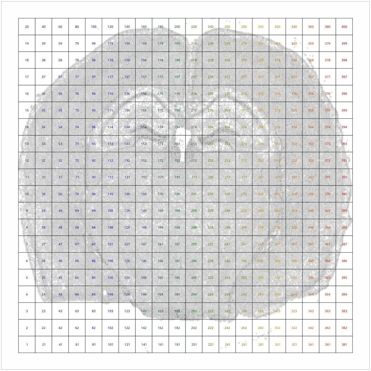
上面的网格图允许我们选择感兴趣的特定区域进行可视化。

hippo = cs.subset_fov(brain, [93, 96, 173, 176],20,20)
x1 = minimum(hippo.x)
x2 = maximum(hippo.x)
y1 = minimum(hippo.y)
y2 = maximum(hippo.y)
cs.sp_dim_plot(brain, "cluster"; anno_color = anno_color,
    do_label = false,marker_size = 7, x_lims = (x1, x2),
    y_lims = (y1, y2),
    width=700, height=600, do_legend=false
    )

​

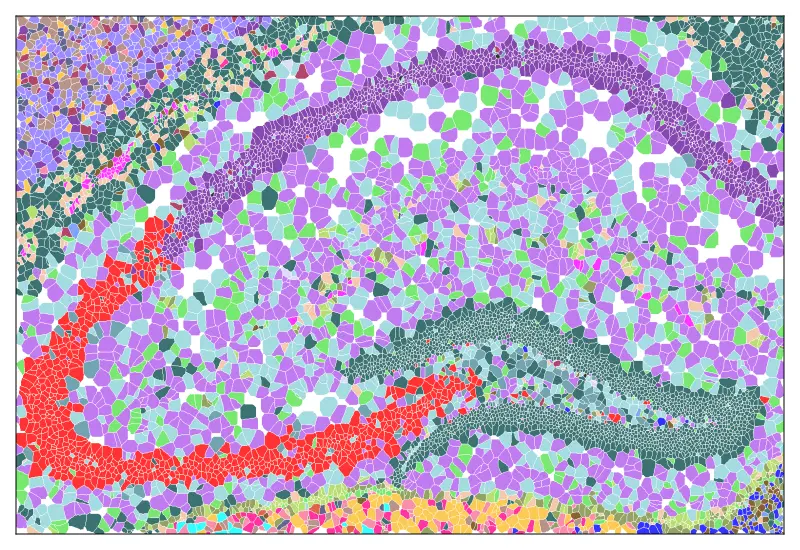
cs.plot_cell_polygons(brain, "cluster"; x_lims = (x1, x2),
    y_lims = (y1, y2), cell_colors= colors, stroke_color="black",
    width = 800, height = 550)

​

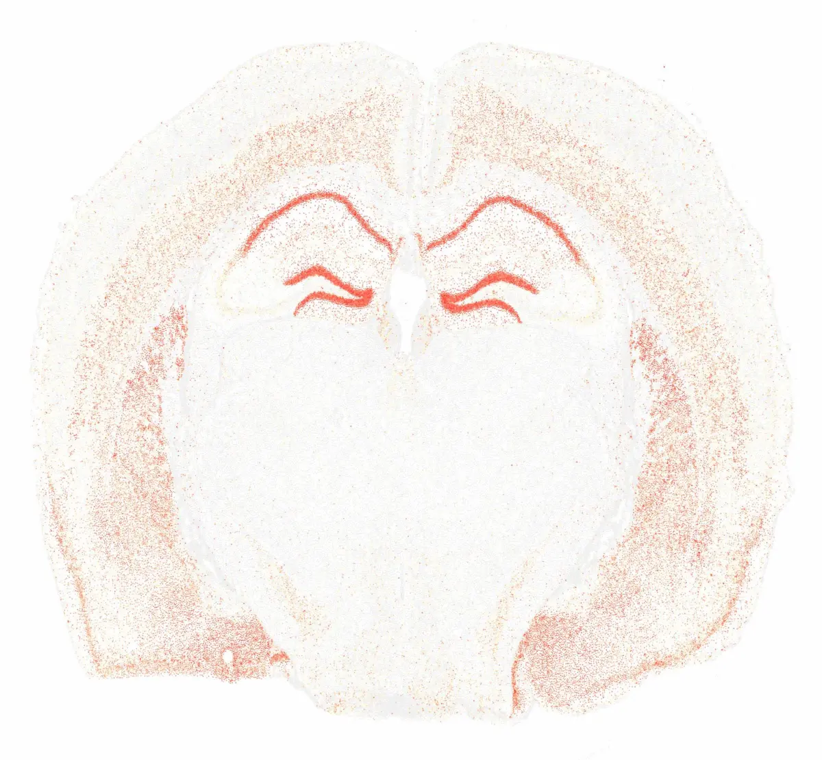
基因可视化

cs.sp_feature_plot(brain, "Bcl11b"; color_keys=["gray94", "lemonchiffon", "red"], height=3000, width=3000, marker_size = 4)

​

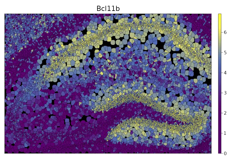
cs.plot_gene_polygons(brain, ["Bcl11b"]; x_lims = (x1, x2),y_lims = (y1, y2),
    width = 800, height = 550, color_keys=["#440154", "#440154","#3b528b","#ffff67"], bg_color="black")

​

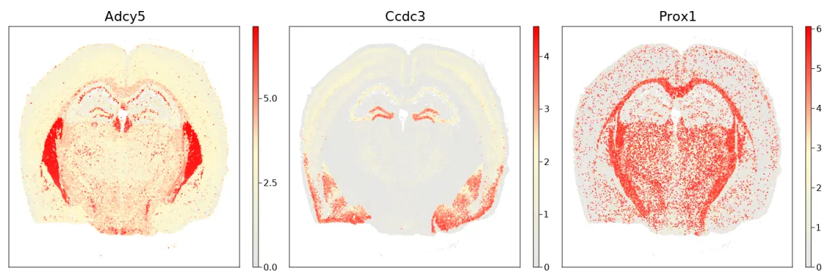
Gene imputation

提供包装函数运行基因插入使用三种不同的工具:SpaGE, gimVI和tangram。

data_path = "/mnt/sdc/new_analysis_cellscopes/brain_sc/"
SpaGE_path = "/mnt/sdc/new_analysis_cellscopes/SpaGE/"
brain = cs.run_spaGE(brain, data_path, SpaGE_path)

cs.sp_feature_plot(brain, ["Adcy5","Ccdc3", "Prox1"]; color_keys=["gray90", "lemonchiffon", "red"], use_imputed = true)

​

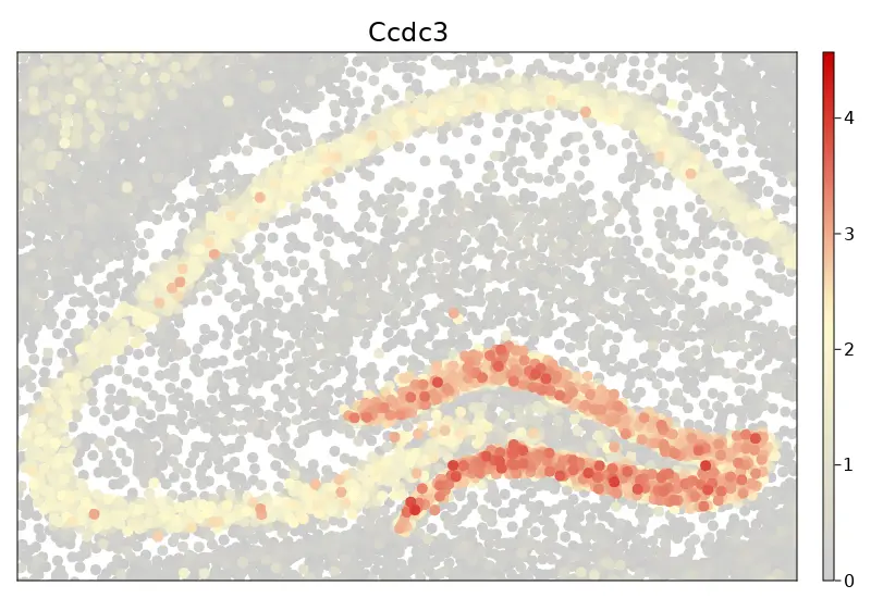
cs.sp_feature_plot(brain2, ["Ccdc3"]; 
    color_keys=["gray80", "lemonchiffon", "red3"], order=true,
    use_imputed = true, x_lims = (x1, x2), marker_size = 10,
    y_lims = (y1, y2),width = 800, height = 550)

​

生活很好，有你更好