DSP(Digital Spatial Profiler)空间转录组与单细胞数据联合分析之cell2location

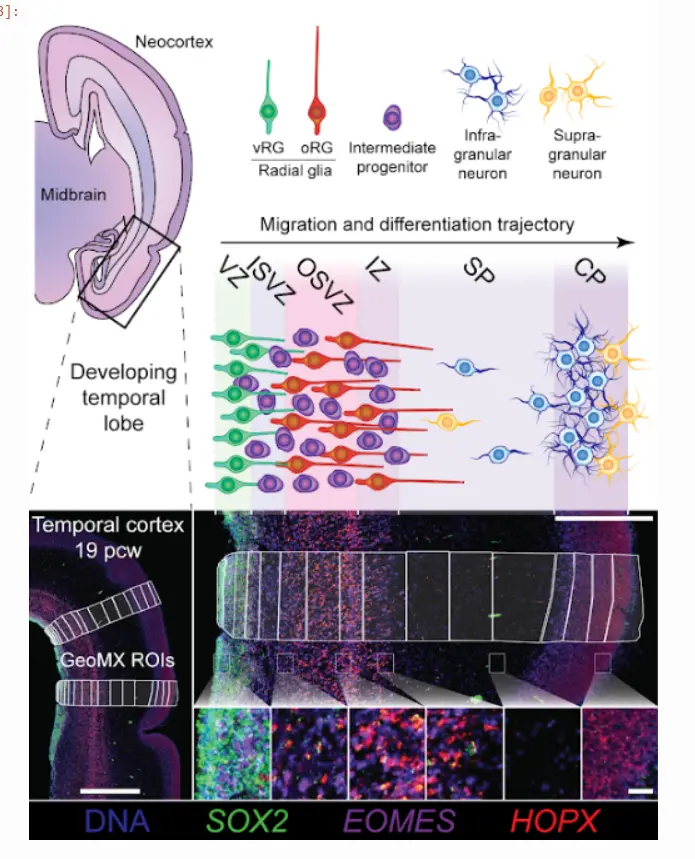
这一篇继续回顾一下cell2location，使用我们推荐用于基于探针的空间转录组学数据的 cell2location 方法的一个版本，将胎儿脑细胞类型映射到使用 NanostringWTA（就是DSP） 技术分析的感兴趣区域 (ROI)。

Load the required modules and configure theano settings:

import sys,os
import pickle
import anndata
import pandas as pd
import numpy as np
import matplotlib.pyplot as plt
import scanpy as sc
from IPython.display import Image
data_type = 'float32'
os.environ["THEANO_FLAGS"] = 'device=cuda,floatX=' + data_type + ',force_device=True' + ',dnn.enabled=False'
import cell2location

# Download data:
os.mkdir('./data')
os.system('cd ./data && wget https://cell2location.cog.sanger.ac.uk/nanostringWTA/nanostringWTA_fetailBrain_AnnData_smallestExample.p')
os.system('cd ./data && wget https://cell2location.cog.sanger.ac.uk/nanostringWTA/polioudakis2019_meanExpressionProfiles.csv')

Load a data:

adata_wta = pickle.load(open("data/nanostringWTA_fetailBrain_AnnData_smallestExample.p", "rb" ))

在此 NanostringWTA 运行中，分析了 288 个感兴趣区域 (ROI)，跨越整个皮层深度以及 19pcw 和 14pcw。 下图显示了一个示例，以及在每个区域中期望的细胞类型：

Image(filename='../images/GeometricROIs.PNG')

Here we load an existing matrix of average gene expression profiles for each cell type expected in our nanostringWTA data (taken from the single-cell RNAseq study Polioudakis et al., Neuron, 2019):

meanExpression_sc = pd.read_csv("data/polioudakis2019_meanExpressionProfiles.csv", index_col=0)

需要单独的基因探针和阴性探针，如果有的话，还可以提供细胞核计数。 在这里初始化所有这些：

counts_negativeProbes = np.asarray(adata_wta[:,np.array(adata_wta.var_names =='NegProbe-WTX').squeeze()].X)
counts_nuclei = np.asarray(adata_wta.obs['nuclei']).reshape(len(adata_wta.obs['nuclei']),1)
adata_wta = adata_wta[:,np.array(adata_wta.var_names != 'NegProbe-WTX').squeeze()]

细胞核计数和负探针需要是 numpy 数组，但基因探针计数作为 AnnData 对象提供。

adata_wta.raw = adata_wta

Run cell2location:

参数解释如下：

• ‘model_name = cell2location.models.LocationModelWTA’ > 这里cell2location使用NanostringWTA模型，而不是标准模型。
• ‘use_raw’: False > 从 adata_wta.X 而不是从 adata_wta.raw.X 中提取数据
• ‘Y_data’: counts_negativeProbes > 我们在这里提供负探针信息
• ‘cell_number_prior’和‘cell_number_var_prior’：在这里提供关于细胞核计数的信息.

cell2location.run_c2l.run_cell2location(meanExpression_sc, adata_wta,
        model_name=cell2location.models.LocationModelWTA,
        train_args={'use_raw': False},
        model_kwargs={
        "Y_data" : counts_negativeProbes,
        "cell_number_prior" : {'cells_per_spot': counts_nuclei, 'factors_per_spot': 6, 'combs_per_spot': 3},
        "cell_number_var_prior" : {'cells_mean_var_ratio': 1, 'factors_mean_var_ratio': 1, 'combs_mean_var_ratio': 1}})

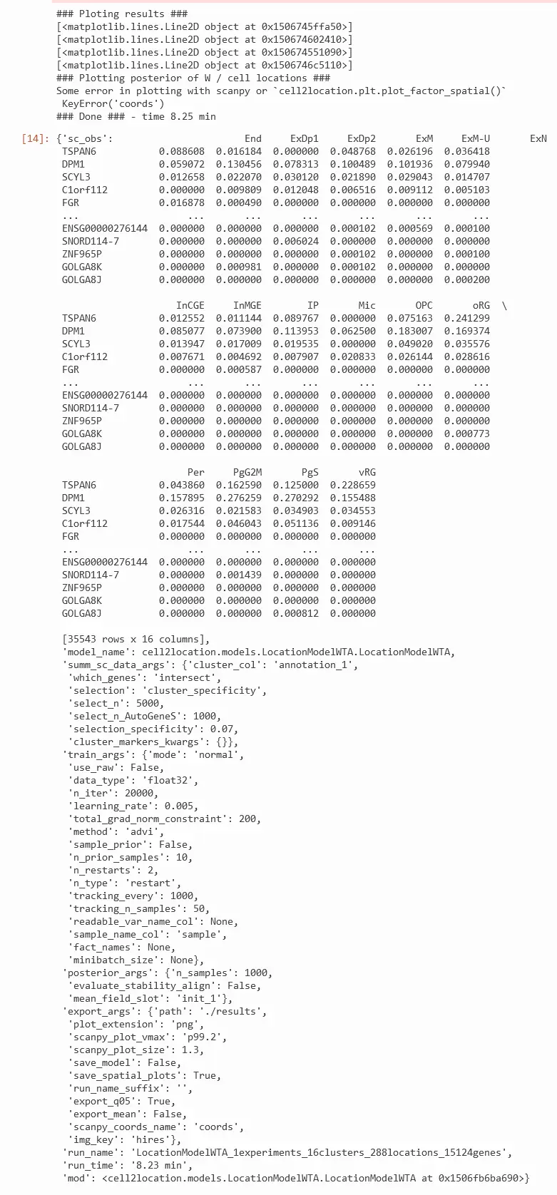
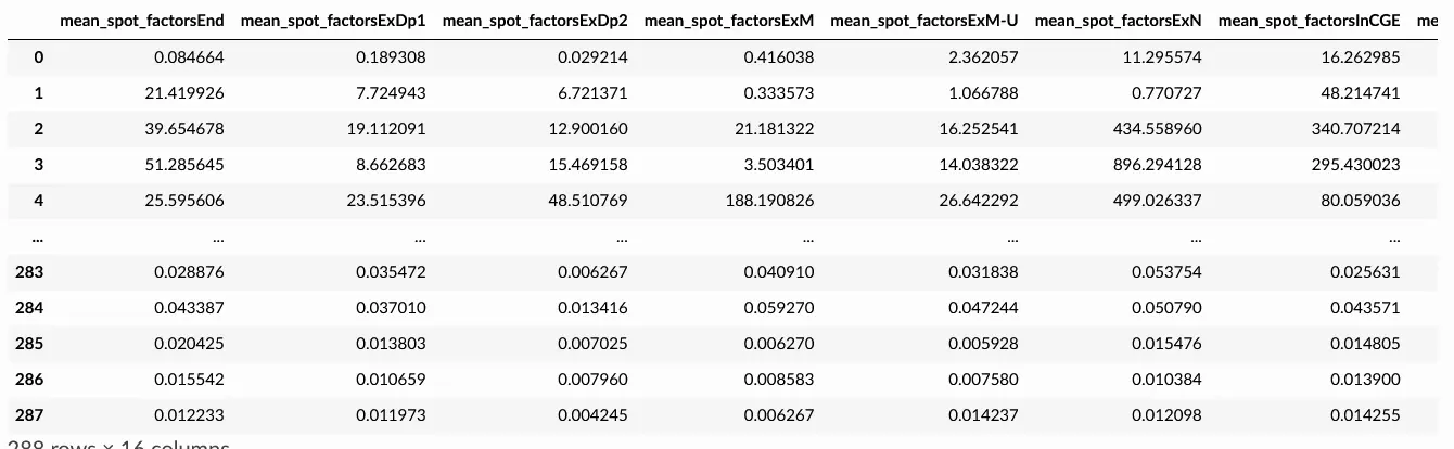
An anndata object that has the cell2location results included is saved and can be used for further analysis, as in standard cell2location:

adata_c2l = sc.read_h5ad('resultsLocationModelWTA_1experiments_16clusters_288locations_15124genes/sp.h5ad')
adata_c2l.obs.loc[:,['mean_spot_factors' in c for c in adata_c2l.obs.columns]]

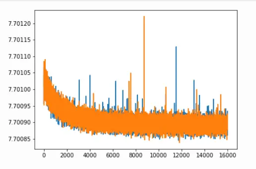
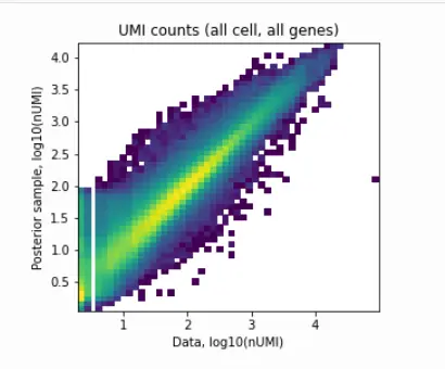
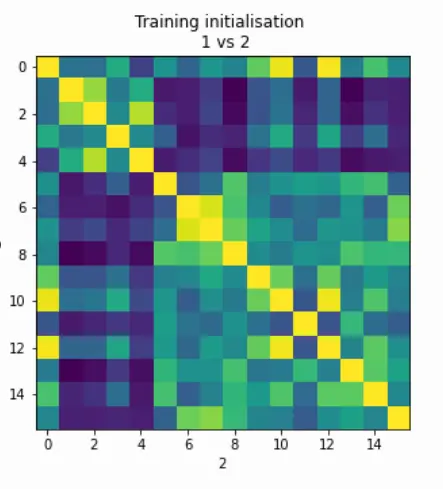
We can also plot the same QC metrics as in standard cell2location:

from IPython.display import Image
Image(filename='resultsLocationModelWTA_1experiments_16clusters_288locations_15124genes/plots/training_history_without_first_20perc.png',
      width=400)

Image(filename='resultsLocationModelWTA_1experiments_16clusters_288locations_15124genes/plots/data_vs_posterior_mean.png',
      width=400)

Image(filename='resultsLocationModelWTA_1experiments_16clusters_288locations_15124genes/plots/evaluate_stability.png',
      width=400)

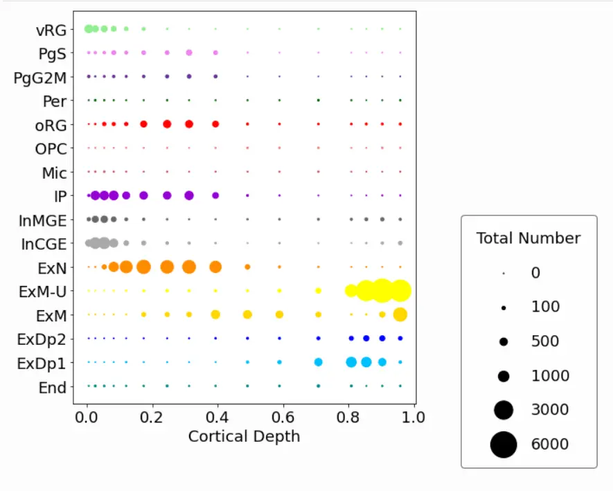
最后，有这种方法可以在我们感兴趣的坐标（皮质深度）上绘制一维细胞类型丰度：

It makes most sense to plot a subset, for example on one 19pcw slide at one position:

colourCode = {'SPN': 'salmon', 'End': 'darkcyan', 'ExDp1': 'deepskyblue', 'ExDp2': 'blue', 'ExM': 'gold', 'ExM-U': 'yellow',
              'ExN': 'darkorange', 'InCGE': 'darkgrey', 'InMGE': 'dimgray', 'IP': 'darkviolet',
              'Mic': 'indianred', 'OPC': 'lightcoral', 'oRG': 'red', 'Per': 'darkgreen',
              'PgG2M': 'rebeccapurple', 'PgS': 'violet', 'vRG': 'lightgreen'}

subset_19pcw = [adata_c2l.obs['slide'].iloc[i] == '00MU' and
         adata_c2l.obs['Radial_position'].iloc[i] == 2 for i in range(len(adata_c2l.obs['Radial_position']))]

cell2location.plt.plot_absolute_abundances_1D(adata_c2l, subset = subset_19pcw, saving = False,
                               scaling = 0.15, power = 1, pws = [0,0,100,500,1000,3000,6000], figureSize = (12,8),
                               dimName = 'VCDepth', xlab = 'Cortical Depth', colourCode = colourCode)

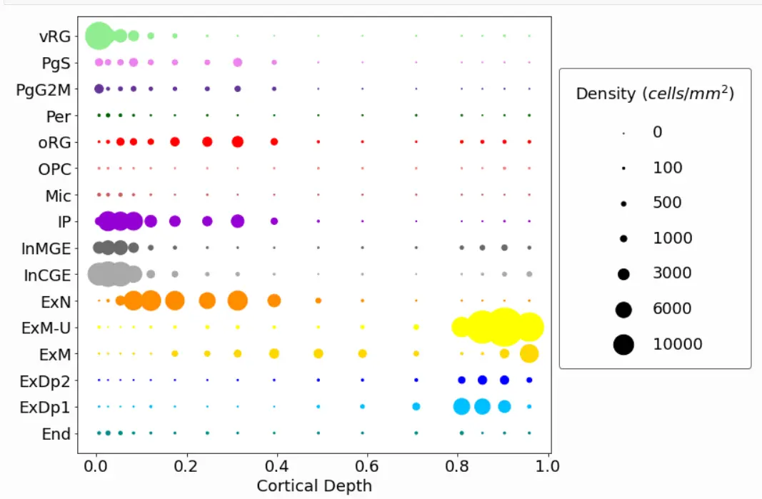
You can also plot density rather than total numbers:

cell2location.plt.plot_density_1D(adata_c2l, subset = subset_19pcw, saving = False,
                               scaling = 0.05, power = 1, pws = [0,0,100,500,1000,3000,6000,10000], figureSize = (12,8),
                               dimName = 'VCDepth', areaName = 'roi_dimension', xlab = 'Cortical Depth',
                colourCode = colourCode)

生活很好，有你更好