


作者,Evil Genius
我们HD部分的授课也要结束了,还是那句话,10X HD数据结合图像分割获取单细胞级别的空间数据,才是10X HD数据分析的更优解,也是各种高精度平台分析的更优解。
介绍
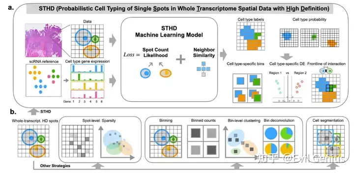
空间转录组学领域旨在捕捉组织完整的转录图谱,并将基因表达映射到特定位置,揭示不同细胞类型的空间分布及其分子活性。10x的Visium分析使用barcodes的载玻片捕获和定位转录表达。在Visium HD空间基因表达实验中,barcodes在2x2um方格内形成网格。除此之外,SpaceRanger pipline cre ates 8x8 um and 16 um的空间表达数据。 Each bin包含多个2x2um正方形的UMI计数的基因总和。这不是整合基因表达数据的唯一方法。另一种方法是使用Visium HD检测中使用的组织的显微镜图像中包含的信息来创建自定义bin。使用从高分辨率H&E图像染色的核,根据barcode对应的核,将barcode划分为bin。barcode被划分成特定于细胞核的bin,模仿单细胞数据,因为基因计数现在将按每个细胞形成。
Two approaches for binning the 2x2 µm barcode squares in Visium HD data
分析要求
- Visium HD基因表达检测中使用的样品高分辨率H&E图像
- Output from a completed Space Ranger count analysis
- 熟悉Python编程
CytAssist 所拍摄的图像不适合于此分析,因为它只是细胞质的伊红染色,缺乏细胞核的血红素染色。
概述
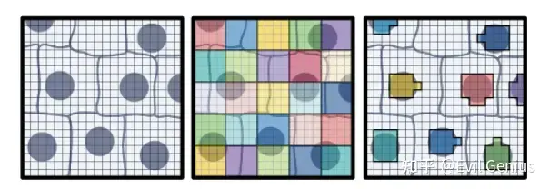
为了生成定制的核特异性bins,首先分割高分辨率的H&E图像以创建nuclei mask。然后,使用mask中每个核的形状和位置将Barcode分类为与每个单独的核相对应的bins。最后,对每个bin中的UMI计数执行求和,从而产生单细胞级别的空间矩阵。
推荐使用StarDist进行图像分割。使用自定义python脚本根据分段的nuclei mask对基因表达数据进行绑定和求和。由此生成的基因分组barcode矩阵非常适合于可视化和下游分析。所有的步骤都是使用python程序设计语言进行的。
Analysis Guide Data Download Links
For this tutorial you will need the following files.
1、2x2 µm filtered barcode matrix ( filtered_feature_bc_matrix.h5)
- This file is located in the /outs/binned_outputs/square_002um directory of a completed Space Ranger run.
- The filtered_feature_bc_matrix.h5 is an HDF5 formatted file where the number of UMIs associated with a feature or gene is stored in the rows of a matrix and each column of the matrix is a barcode.
2、Parquet tissue position matrix (tissue_positions.parquet) - This files is located in the /outs/binned_outputs/square_002um/spatial directory of a completed Space Ranger run.
- The tissue_positions.parquet file contains a table of the location of each 2x2 µm barcode square where each column is a barcode.
3、High-resolution mouse intestine image (Visium_HD_Mouse_Small_Intestine_tissue_image.btf) - This is an image generated by the user using a microscope.
- The name and location of this file is user defined.
- The time to transfer a high-resolution image can vary depending on internet access, and it may take a significant amount of time due to the file's size.
示例数据下载
curl -O https://cf.10xgenomics.com/samples/spatial-exp/3.0.0/Visium_HD_Mouse_Small_Intestine/Visium_HD_Mouse_Small_Intestine_binned_outputs.tar.gz
curl -O https://cf.10xgenomics.com/samples/spatial-exp/3.0.0/Visium_HD_Mouse_Small_Intestine/Visium_HD_Mouse_Small_Intestine_tissue_image.btf
软件安装
Important Python Libraries
stardist is a deep-learning library for star-convex object detection of cells/nuclei.
geopandas is an extension of the pandas library for working with geospatial data.
squidpy is a collection of tools that are built on scanpy and anndata for the visualization and analysis of spatial gene expression data. It is used in this guide mainly for the scanpy and anndata libraries.
fastparquet is a Python library for efficient reading and writing of Apache Parquet files.
使用conda安装
# Update conda
conda update conda

# Create the conda environment, add the conda-forge channel, and set channel priority.
conda create -n stardist-env

# Activate the environment
conda activate stardist-env
conda config --env --add channels conda-forge
conda config --env --set channel_priority strict


# Install Python libraries
conda install -c conda-forge stardist
conda install python=3 geopandas
conda install -c conda-forge squidpy
conda install -c conda-forge fastparquet
模块加载
import pandas as pd
import numpy as np
import matplotlib.pyplot as plt
import anndata
import geopandas as gpd
import scanpy as sc

from tifffile import imread, imwrite
from csbdeep.utils import normalize
from stardist.models import StarDist2D
from shapely.geometry import Polygon, Point
from scipy import sparse
from matplotlib.colors import ListedColormap

%matplotlib inline
%config InlineBackend.figure_format = 'retina'
数据可视化的函数定义
# General image plotting functions
def plot_mask_and_save_image(title, gdf, img, cmap, output_name=None, bbox=None):
    if bbox is not None:
        # Crop the image to the bounding box
        cropped_img = img[bbox[1]:bbox[3], bbox[0]:bbox[2]]
    else:
        cropped_img = img

    # Plot options
    fig, axes = plt.subplots(1, 2, figsize=(12, 6))

    # Plot the cropped image
    axes[0].imshow(cropped_img, cmap='gray', origin='lower')
    axes[0].set_title(title)
    axes[0].axis('off')

    # Create filtering polygon
    if bbox is not None:
        bbox_polygon = Polygon([(bbox[0], bbox[1]), (bbox[2], bbox[1]), (bbox[2], bbox[3]), (bbox[0], bbox[3])])
        # Filter for polygons in the box
        intersects_bbox = gdf['geometry'].intersects(bbox_polygon)
        filtered_gdf = gdf[intersects_bbox]
    else:
        filtered_gdf=gdf

    # Plot the filtered polygons on the second axis
    filtered_gdf.plot(cmap=cmap, ax=axes[1])
    axes[1].axis('off')
    axes[1].legend(loc='upper left', bbox_to_anchor=(1.05, 1))


    # Save the plot if output_name is provided
    if output_name is not None:
        plt.savefig(output_name, bbox_inches='tight')  # Use bbox_inches='tight' to include the legend
    else:
        plt.show()

def plot_gene_and_save_image(title, gdf, gene, img, adata, bbox=None, output_name=None):

    if bbox is not None:
        # Crop the image to the bounding box
        cropped_img = img[bbox[1]:bbox[3], bbox[0]:bbox[2]]
    else:
        cropped_img = img

    # Plot options
    fig, axes = plt.subplots(1, 2, figsize=(12, 6))

    # Plot the cropped image
    axes[0].imshow(cropped_img, cmap='gray', origin='lower')
    axes[0].set_title(title)
    axes[0].axis('off')

    # Create filtering polygon
    if bbox is not None:
        bbox_polygon = Polygon([(bbox[0], bbox[1]), (bbox[2], bbox[1]), (bbox[2], bbox[3]), (bbox[0], bbox[3])])


    # Find a gene of interest and merge with the geodataframe
    gene_expression = adata[:, gene].to_df()
    gene_expression['id'] = gene_expression.index
    merged_gdf = gdf.merge(gene_expression, left_on='id', right_on='id')

    if bbox is not None:
        # Filter for polygons in the box
        intersects_bbox = merged_gdf['geometry'].intersects(bbox_polygon)
        filtered_gdf = merged_gdf[intersects_bbox]
    else:
        filtered_gdf = merged_gdf

    # Plot the filtered polygons on the second axis
    filtered_gdf.plot(column=gene, cmap='inferno', legend=True, ax=axes[1])
    axes[1].set_title(gene)
    axes[1].axis('off')
    axes[1].legend(loc='upper left', bbox_to_anchor=(1.05, 1))

    # Save the plot if output_name is provided
    if output_name is not None:
        plt.savefig(output_name, bbox_inches='tight')  # Use bbox_inches='tight' to include the legend
    else:
        plt.show()

def plot_clusters_and_save_image(title, gdf, img, adata, bbox=None, color_by_obs=None, output_name=None, color_list=None):
    color_list=["#7f0000","#808000","#483d8b","#008000","#bc8f8f","#008b8b","#4682b4","#000080","#d2691e","#9acd32","#8fbc8f","#800080","#b03060","#ff4500","#ffa500","#ffff00","#00ff00","#8a2be2","#00ff7f","#dc143c","#00ffff","#0000ff","#ff00ff","#1e90ff","#f0e68c","#90ee90","#add8e6","#ff1493","#7b68ee","#ee82ee"]
    if bbox is not None:
        cropped_img = img[bbox[1]:bbox[3], bbox[0]:bbox[2]]
    else:
        cropped_img = img

    fig, axes = plt.subplots(1, 2, figsize=(12, 6))

    axes[0].imshow(cropped_img, cmap='gray', origin='lower')
    axes[0].set_title(title)
    axes[0].axis('off')

    if bbox is not None:
        bbox_polygon = Polygon([(bbox[0], bbox[1]), (bbox[2], bbox[1]), (bbox[2], bbox[3]), (bbox[0], bbox[3])])

    unique_values = adata.obs[color_by_obs].astype('category').cat.categories
    num_categories = len(unique_values)

    if color_list is not None and len(color_list) >= num_categories:
        custom_cmap = ListedColormap(color_list[:num_categories], name='custom_cmap')
    else:
        # Use default tab20 colors if color_list is insufficient
        tab20_colors = plt.cm.tab20.colors[:num_categories]
        custom_cmap = ListedColormap(tab20_colors, name='custom_tab20_cmap')

    merged_gdf = gdf.merge(adata.obs[color_by_obs].astype('category'), left_on='id', right_index=True)

    if bbox is not None:
        intersects_bbox = merged_gdf['geometry'].intersects(bbox_polygon)
        filtered_gdf = merged_gdf[intersects_bbox]
    else:
        filtered_gdf = merged_gdf

    # Plot the filtered polygons on the second axis
    plot = filtered_gdf.plot(column=color_by_obs, cmap=custom_cmap, ax=axes[1], legend=True)
    axes[1].set_title(color_by_obs)
    legend = axes[1].get_legend()
    legend.set_bbox_to_anchor((1.05, 1))
    axes[1].axis('off')

    # Move legend outside the plot
    plot.get_legend().set_bbox_to_anchor((1.25, 1))

    if output_name is not None:
        plt.savefig(output_name, bbox_inches='tight')
    else:
        plt.show()

# Plotting function for nuclei area distribution
def plot_nuclei_area(gdf,area_cut_off):
    fig, axs = plt.subplots(1, 2, figsize=(15, 4))
    # Plot the histograms
    axs[0].hist(gdf['area'], bins=50, edgecolor='black')
    axs[0].set_title('Nuclei Area')

    axs[1].hist(gdf[gdf['area'] < area_cut_off]['area'], bins=50, edgecolor='black')
    axs[1].set_title('Nuclei Area Filtered:'+str(area_cut_off))

    plt.tight_layout()
    plt.show()

# Total UMI distribution plotting function
def total_umi(adata_, cut_off):
    fig, axs = plt.subplots(1, 2, figsize=(12, 4))

    # Box plot
    axs[0].boxplot(adata_.obs["total_counts"], vert=False, widths=0.7, patch_artist=True, boxprops=dict(facecolor='skyblue'))
    axs[0].set_title('Total Counts')

    # Box plot after filtering
    axs[1].boxplot(adata_.obs["total_counts"][adata_.obs["total_counts"] > cut_off], vert=False, widths=0.7, patch_artist=True, boxprops=dict(facecolor='skyblue'))
    axs[1].set_title('Total Counts > ' + str(cut_off))

    # Remove y-axis ticks and labels
    for ax in axs:
        ax.get_yaxis().set_visible(False)

    plt.tight_layout()
    plt.show()
Nuclei Mask and GeoDataframe Creation
将文件路径更改为高分辨率图像的位置。导入图像后,它会进行百分位归一化。通过评估图像mask的准确性来调整其他图像所需的min和max百分位参数。百分位归一化通过指定的min和max百分位来缩放像素值。
# Load the image file
# Change dir_base as needed to the directory where the downloaded example data is stored
dir_base = '/path_to_data/'
filename = 'SJ0309_MsSI_slide08_01_20x_BF_01.btf'
img = imread(dir_base + filename)

# Load the pretrained model
model = StarDist2D.from_pretrained('2D_versatile_he')

# Percentile normalization of the image
# Adjust min_percentile and max_percentile as needed
min_percentile = 5
max_percentile = 95
img = normalize(img, min_percentile, max_percentile)
执行下面的代码以创建核分割mask。此步骤运行时间较长,并且它将根据所选参数设置而显著变化。nms阈值(nms thresh)设置为小数,以减少核重叠的概率。nms thresh参数可能需要根据不同的图像进行调整。此外,可能需要根据不同的图像调整概率阈值(prob thresh)。较大的prob_thresh值将导致较少的分割对象。prob_thresh和nms thresh的最佳值将取决于核分割mask的视觉评估。
# Predict cell nuclei using the normalized image
# Adjust nms_thresh and prob_thresh as needed

labels, polys = model.predict_instances_big(img, axes='YXC', block_size=4096, prob_thresh=0.01,nms_thresh=0.001, min_overlap=128, context=128, normalizer=None, n_tiles=(4,4,1))
The function predict_instances_big divides the input image into blocks, processes them individually using predict_instances, and then combines the results.
将StarDist的结果转换为 Geodataframe。将使用 Geodataframe进行barcode排序
# Creating a list to store Polygon geometries
geometries = []

# Iterating through each nuclei in the 'polys' DataFrame
for nuclei in range(len(polys['coord'])):

    # Extracting coordinates for the current nuclei and converting them to (y, x) format
    coords = [(y, x) for x, y in zip(polys['coord'][nuclei][0], polys['coord'][nuclei][1])]

    # Creating a Polygon geometry from the coordinates
    geometries.append(Polygon(coords))

# Creating a GeoDataFrame using the Polygon geometries
gdf = gpd.GeoDataFrame(geometry=geometries)
gdf['id'] = [f"ID_{i+1}" for i, _ in enumerate(gdf.index)]为了可视化的分割结果,将从高分辨率的H&E图像中选择一个感兴趣的区域,并定义一个限界框。限界框描绘感兴趣区域的边界。选择一个较小的区域的图像,能够放大和检查的细胞核更仔细的分割。
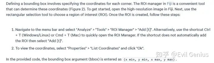
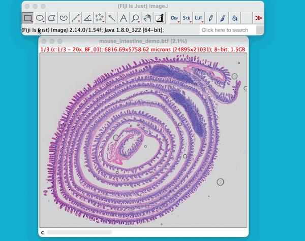
选定好坐标以后,框选区域
# Plot the nuclei segmentation
# bbox=(x min,y min,x max,y max)

# Define a single color cmap
cmap=ListedColormap(['grey'])

# Create Plot
plot_mask_and_save_image(title="Region of Interest 1",gdf=gdf,bbox=(12844,7700,13760,8664),cmap=cmap,img=img,output_name=dir_base+"image_mask.ROI1.tif")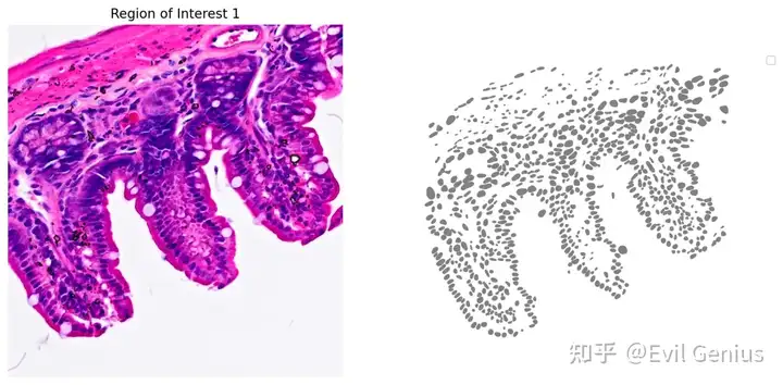
Binning Visium HD Gene Expression Data
加载了2x2 um Visium HD基因表达数据和组织位置信息,然后创建了一个GeoDataFrame。请确保表达数据和组织位置文件与高分辨率H&E显微镜图像在同一目录中。
# Load Visium HD data
raw_h5_file = dir_base+'filtered_feature_bc_matrix.h5'
adata = sc.read_10x_h5(raw_h5_file)

# Load the Spatial Coordinates
tissue_position_file = dir_base+'tissue_positions.parquet'
df_tissue_positions=pd.read_parquet(tissue_position_file)

#Set the index of the dataframe to the barcodes
df_tissue_positions = df_tissue_positions.set_index('barcode')

# Create an index in the dataframe to check joins
df_tissue_positions['index']=df_tissue_positions.index

# Adding the tissue positions to the meta data
adata.obs =  pd.merge(adata.obs, df_tissue_positions, left_index=True, right_index=True)

# Create a GeoDataFrame from the DataFrame of coordinates
geometry = [Point(xy) for xy in zip(df_tissue_positions['pxl_col_in_fullres'], df_tissue_positions['pxl_row_in_fullres'])]
gdf_coordinates = gpd.GeoDataFrame(df_tissue_positions, geometry=geometry)
检查每个条形码,以确定它们是否在细胞核中。有两个或多个细胞核重叠的可能性,因此,为了消除条形码分配的歧义,稍后将过滤掉,只保留唯一分配的条形码。
# Perform a spatial join to check which coordinates are in a cell nucleus
result_spatial_join = gpd.sjoin(gdf_coordinates, gdf, how='left', predicate='within')

# Identify nuclei associated barcodes and find barcodes that are in more than one nucleus
result_spatial_join['is_within_polygon'] = ~result_spatial_join['index_right'].isna()
barcodes_in_overlaping_polygons = pd.unique(result_spatial_join[result_spatial_join.duplicated(subset=['index'])]['index'])
result_spatial_join['is_not_in_an_polygon_overlap'] = ~result_spatial_join['index'].isin(barcodes_in_overlaping_polygons)

# Remove barcodes in overlapping nuclei
barcodes_in_one_polygon = result_spatial_join[result_spatial_join['is_within_polygon'] & result_spatial_join['is_not_in_an_polygon_overlap']]

# The AnnData object is filtered to only contain the barcodes that are in non-overlapping polygon regions
filtered_obs_mask = adata.obs_names.isin(barcodes_in_one_polygon['index'])
filtered_adata = adata[filtered_obs_mask,:]

# Add the results of the point spatial join to the Anndata object
filtered_adata.obs =  pd.merge(filtered_adata.obs, barcodes_in_one_polygon[['index','geometry','id','is_within_polygon','is_not_in_an_polygon_overlap']], left_index=True, right_index=True)
获取单细胞级别的空间数据
# Group the data by unique nucleous IDs
groupby_object = filtered_adata.obs.groupby(['id'], observed=True)

# Extract the gene expression counts from the AnnData object
counts = filtered_adata.X

# Obtain the number of unique nuclei and the number of genes in the expression data
N_groups = groupby_object.ngroups
N_genes = counts.shape[1]

# Initialize a sparse matrix to store the summed gene counts for each nucleus
summed_counts = sparse.lil_matrix((N_groups, N_genes))

# Lists to store the IDs of polygons and the current row index
polygon_id = []
row = 0

# Iterate over each unique polygon to calculate the sum of gene counts.
for polygons, idx_ in groupby_object.indices.items():
    summed_counts[row] = counts[idx_].sum(0)
    row += 1
    polygon_id.append(polygons)

# Create and AnnData object from the summed count matrix
summed_counts = summed_counts.tocsr()
grouped_filtered_adata = anndata.AnnData(X=summed_counts,obs=pd.DataFrame(polygon_id,columns=['id'],index=polygon_id),var=filtered_adata.var)

###store grouped_filtered_adata
Nuclei Binning Results(核过滤是可选的)
# Store the area of each nucleus in the GeoDataframe
gdf['area'] = gdf['geometry'].area

# Calculate quality control metrics for the original AnnData object
sc.pp.calculate_qc_metrics(grouped_filtered_adata, inplace=True)

# Plot the nuclei area distribution before and after filtering
plot_nuclei_area(gdf=gdf,area_cut_off=500)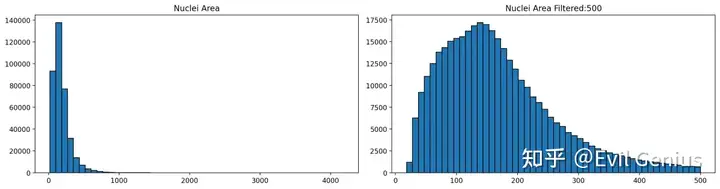
接下来就是类似单细胞数据的处理了
Based on the nuclei distribution we selected a value of 500 to filter the data.
# Create a mask based on the 'id' column for values present in 'gdf' with 'area' less than 500
mask_area = grouped_filtered_adata.obs['id'].isin(gdf[gdf['area'] < 500].id)

# Create a mask based on the 'total_counts' column for values greater than 100
mask_count = grouped_filtered_adata.obs['total_counts'] > 100

# Apply both masks to the original AnnData to create a new filtered AnnData object
count_area_filtered_adata = grouped_filtered_adata[mask_area & mask_count, :]

# Calculate quality control metrics for the filtered AnnData object
sc.pp.calculate_qc_metrics(count_area_filtered_adata, inplace=True)
为了评估binning结果,检查基因表达和聚类。
# Normalize total counts for each cell in the AnnData object
sc.pp.normalize_total(count_area_filtered_adata, inplace=True)

# Logarithmize the values in the AnnData object after normalization
sc.pp.log1p(count_area_filtered_adata)

# Identify highly variable genes in the dataset using the Seurat method
sc.pp.highly_variable_genes(count_area_filtered_adata, flavor="seurat", n_top_genes=2000)

# Perform Principal Component Analysis (PCA) on the AnnData object
sc.pp.pca(count_area_filtered_adata)

# Build a neighborhood graph based on PCA components
sc.pp.neighbors(count_area_filtered_adata)

# Perform Leiden clustering on the neighborhood graph and store the results in 'clusters' column

# Adjust the resolution parameter as needed for different samples
sc.tl.leiden(count_area_filtered_adata, resolution=0.35, key_added="clusters")

# Plot and save the clustering results
plot_clusters_and_save_image(title="Region of interest 1", gdf=gdf, img=img, adata=count_area_filtered_adata, bbox=(12844,7700,13760,8664), color_by_obs='clusters', output_name=dir_base+"image_clustering.ROI1.tiff")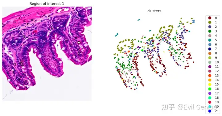
marker基因表达示例
# Plot Lyz1 gene expression
plot_gene_and_save_image(title="Region of interest 1", gdf=gdf, gene='Lyz1', img=img, adata=count_area_filtered_adata, bbox=(12844,7700,13760,8664),output_name=dir_base+"image_Lyz1.ROI1.tiff")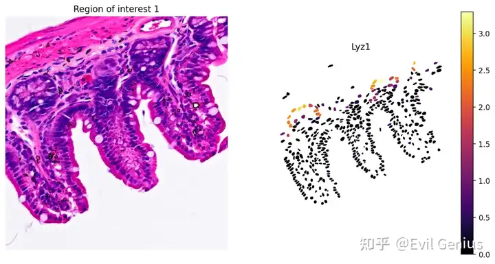
# Plot Muc2 gene expression
plot_gene_and_save_image(title="Region of interest 1", gdf=gdf, gene='Muc2', img=img, adata=count_area_filtered_adata, bbox=(12844,7700,13760,8664),output_name=dir_base+"image_Muc2.ROI1.tiff")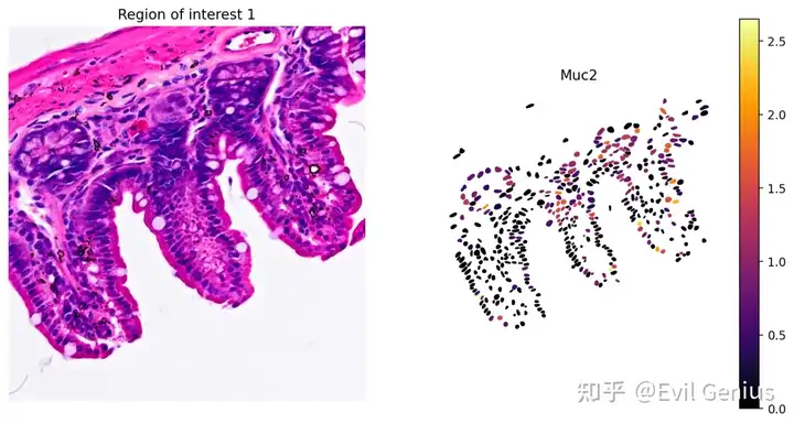
# Plot Fabp2 expression
plot_gene_and_save_image(title="Region of interest 1", gdf=gdf, gene='Fabp2', img=img, adata=count_area_filtered_adata, bbox=(12844,7700,13760,8664),output_name=dir_base+"image_Fabp2.ROI1.tiff")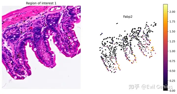
讨论
通过观察与组织形态学相匹配的标记表达和聚类来验证结果。这种方法对于具有清晰定义的大细胞核且易于区分彼此和背景的图像最为有效。对于任何新的H&E切片和Visium HD 基因表达数据集,可能都需要对参数进行优化。需要牢记的关键参数是概率阈值、聚类分辨率以及总 UMI和细胞核大小过滤器截止值。
除了参数优化外,该方法还有一些改进可以提高结果。在示例使用了StarDist的预训练H&E分类器模型。这超出了本分析指南的范围,但 starDist 可以使用自定义训练模型。此外,示例只考虑了核信息。在核mask中扩展每个单独核的边界可以提高结果。


 被折叠的 条评论
为什么被折叠?
被折叠的 条评论
为什么被折叠?
 到【灌水乐园】发言


