


##################多项式拟合预测#################

#多项式拟合,拟合次数n=3,data['week']为time:x数据;data['T5']:y轴数据,需要预测的数据
coefficients = np.polyfit(data['week'], data['T5'], 3)

#将拟合系数数组转换为一个多项式对象
polynomial = np.poly1d(coefficients)

# 预测第0周,对x值为0的位置进行预测
pred5_0 = polynomial(0)

# 添加方程:y=ax^3 + bx^2 + cx + d。,并且保留三位小数
equation = f'y={coefficients[0]:.3f}x^3 {coefficients[1]:.3f}x^2 {coefficients[2]:.3f}x + {coefficients[3]:.3f}'

#输出x值为0的位置的预测值
print(np.around(pred5_0,3))

# 计算拟合误差
fit_error = np.abs(data - polynomial(data['week']))
error = np.around(np.mean(fit_error),3)

# 输出平均拟合误差
print("平均拟合误差:")
print("T5:", error)

#plot
#设置图形
font = {
    'family': 'STSong',
    'serif': 'Times New Roman',
    'weight': '660',
    'size': 18}
plt.rc('font', **font)
plt.style.use('ggplot')
plt.figure(facecolor='white',figsize=(12,6),dpi=300)


x = np.linspace(0, 14, 100)  ##这里的14是时间的长度,100为模拟的点的个数,越多越平滑
y5 = polynomial(x)
plt.scatter(data['week'], data['T5'], color='blue',marker='*', label='原始数据')
plt.plot(x5, y5, color='red',linewidth=1, label='拟合曲线')
plt.scatter(0, pred5_0, color='green', label='预测值')

#在图上添加方程,(2, 200)表示方程在图中的坐标。ha='left':表示方程的中间在该坐标处
plt.text(2, 200, equation5, fontsize=13, ha='left')
#在图上添加误差
plt.text(10, 180, f'Error = {err_T5}', fontsize=13, ha='center')
plt.set_xlabel('周数')
plt.set_ylabel('预定人数')
plt.set_title('航次5',fontsize=18)
plt.xaxis.label.set_fontsize(18)
plt.yaxis.label.set_fontsize(18)

#在图的(-0.1, 1.05)位置添加'a'
plt.text(-0.1, 1.05, 'a', transform=axes[0, 0].transAxes, size=23, weight='bold')
#plt.legend(loc='upper right')##图例的位置
导入数据
import pandas as pd
from pandas import Series
import numpy as np
import matplotlib.pyplot as plt
from sklearn.metrics import mean_absolute_error
#from sklearn.metrics import mean_absolute_percentage_error as mape
import os
from statsmodels.tsa.arima_model import ARIMA
import seaborn as sns
from pmdarima import auto_arima
import statsmodels.api as s
import warnings
warnings.filterwarnings("ignore")#忽略警告
plt.rcParams['font.sans-serif']='SimHei'#设置字体为SimHei
plt.rcParams['axes.unicode_minus']=False#解决负号"-"显示异常
data = pd.read_excel(r"邮轮.xlsx",sheet_name="T")
多项式拟合(六个变量分别预测)
###################T5########################
coefficients5 = np.polyfit(data['week'][0:14,], data['T5'][0:14].values, 3)
polynomial5 = np.poly1d(coefficients5)
# 预测第0周
pred5_0 = polynomial5(0)
# 添加方程
equation5 = f'y={coefficients5[0]:.3f}x^3 {coefficients5[1]:.3f}x^2 {coefficients5[2]:.3f}x + {coefficients5[3]:.3f}'

###################T6#######################
coefficients6 = np.polyfit(data['week'][0:13,], data['T6'][0:13], 3)
polynomial6 = np.poly1d(coefficients6)
# 预测第0
pred6_0 = polynomial6(0)
pred6_1 = polynomial6(1)
# 添加方程
equation6 = f'y={coefficients6[0]:.3f}x^3 + {coefficients6[1]:.3f}x^2 {coefficients6[2]:.3f}x + {coefficients6[3]:.3f}'

###################T7#######################
coefficients7 = np.polyfit(data['week'][0:12,], data['T7'][0:12,], 3)
polynomial7 = np.poly1d(coefficients7)
# 预测第0
pred7_0 = polynomial7(0)
pred7_1 = polynomial7(1)
pred7_2 = polynomial7(2)
# 添加方程
equation7 = f'y={coefficients7[0]:.3f}x^3 + {coefficients7[1]:.3f}x^2 {coefficients7[2]:.3f}x + {coefficients7[3]:.3f}'

###################T8#######################
coefficients8 = np.polyfit(data['week'][0:11,], data['T8'][0:11,], 3)
polynomial8 = np.poly1d(coefficients8)
# 预测第0
pred8_0 = polynomial8(0)
pred8_1 = polynomial8(1)
pred8_2 = polynomial8(2)
pred8_3 = polynomial8(3)
# 添加方程
equation8 = f'y={coefficients8[0]:.3f}x^3 + {coefficients8[1]:.3f}x^2 {coefficients8[2]:.3f}x + {coefficients8[3]:.3f}'

###################T9#######################
coefficients9 = np.polyfit(data['week'][0:10,], data['T9'][0:10,], 3)
polynomial9 = np.poly1d(coefficients9)
# 预测第0
pred9_0 = polynomial9(0)
pred9_1 = polynomial9(1)
pred9_2 = polynomial9(2)
pred9_3 = polynomial9(3)
pred9_4 = polynomial9(4)
# 添加方程
equation9 = f'y={coefficients9[0]:.3f}x^3 + {coefficients9[1]:.3f}x^2 {coefficients9[2]:.3f}x + {coefficients9[3]:.3f}'

###################T10#######################
coefficients10 = np.polyfit(data['week'][0:9,], data['T10'][0:9,], 3)
polynomial10 = np.poly1d(coefficients10)
# 预测第0
pred10_0 = polynomial10(0)
pred10_1 = polynomial10(1)
pred10_2 = polynomial10(2)
pred10_3 = polynomial10(3)
pred10_4 = polynomial10(4)
pred10_5 = polynomial10(5)
# 添加方程
equation10 = f'y={coefficients10[0]:.3f}x^3 + {coefficients10[1]:.3f}x^2 {coefficients10[2]:.3f}x + {coefficients10[3]:.3f}'

#输出结果
print(np.around(pred5_0,3))
print(np.around(pred6_0,3),np.around(pred6_1,3))
print(np.around(pred7_0,3),np.around(pred7_1,3),np.around(pred7_2,3))
print(np.around(pred8_0,3),np.around(pred8_1,3),np.around(pred8_2,3),np.around(pred8_3,3))
print(np.around(pred9_0,3),np.around(pred9_1,3),np.around(pred9_2,3),np.around(pred9_3,3),np.around(pred9_4,3))
print(np.around(pred10_0,3),np.around(pred10_1,3),np.around(pred10_2,3),np.around(pred10_3,3),np.around(pred10_4,3),np.around(pred10_5,3))
计算误差
# 计算拟合误差
fit_error_T5 = np.abs(data['T5'] - polynomial5(data['week']))
err_T5 = np.around(np.mean(fit_error_T5),3)

fit_error_T6 = np.abs(data['T6'][0:13,] - polynomial6(data['week'][0:13,]))
err_T6 = np.around(np.mean(fit_error_T6),3)

fit_error_T7 = np.abs(data['T7'][0:12,] - polynomial7(data['week'][0:12,]))
err_T7 = np.around(np.mean(fit_error_T7),3)

fit_error_T8 = np.abs(data['T8'][0:11,] - polynomial8(data['week'][0:11,]))
err_T8 = np.around(np.mean(fit_error_T8),3)

fit_error_T9 = np.abs(data['T9'][0:10,] - polynomial9(data['week'][0:10,]))
err_T9 = np.around(np.mean(fit_error_T9),3)

fit_error_T10 = np.abs(data['T10'][0:9,] - polynomial10(data['week'][0:9,]))
err_T10 = np.around(np.mean(fit_error_T10),3)

# 输出平均拟合误差
print("平均拟合误差:")
print("T5:", err_T5)
print("T6:", err_T6)
print("T7:", err_T7)
print("T8:", err_T8)
print("T9:", err_T9)
print("T10:", err_T10)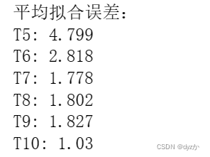
可视化
font = {
    'family': 'STSong',
    'serif': 'Times New Roman',
    'weight': '660',
    'size': 18}
plt.rc('font', **font)
plt.style.use('ggplot')
plt.figure(facecolor='white',figsize=(12,6),dpi=300)

###################T5
fig, axes = plt.subplots(nrows=2, ncols=3, figsize=(16, 8),dpi=300)
plt.rcParams["font.weight"] = "bold"
###############################################
x = np.linspace(0, 14, 100)
y5 = polynomial5(x)
axes[0, 0].scatter(data['week'], data['T5'], color='blue',marker='*', label='原始数据')
axes[0, 0].plot(x5, y5, color='red',linewidth=1, label='拟合曲线')
axes[0, 0].scatter(0, pred5_0, color='green', label='预测值')
axes[0, 0].text(2, 200, equation5, fontsize=13, ha='left')
axes[0, 0].text(10, 180, f'Error = {err_T5}', fontsize=13, ha='center')
# axes[0, 0].set_xlabel('周数')
axes[0, 0].set_ylabel('预定人数')
axes[0, 0].set_title('航次5',fontsize=18)
axes[0, 0].xaxis.label.set_fontsize(18)
axes[0, 0].yaxis.label.set_fontsize(18)
axes[0, 0].text(-0.1, 1.05, 'a', transform=axes[0, 0].transAxes, size=23, weight='bold')
# axes[0, 0].legend(loc='upper right')
###############################################
axes[0, 1].scatter(data['week'][0:13,], data['T6'][0:13], color='blue',marker='*', label='原始数据')
axes[0, 1].plot(np.linspace(0, 14, 100), polynomial6(x), color='red',linewidth=1, label='拟合曲线')
axes[0, 1].scatter([0,1], [pred6_0,pred6_1], color='green', label='预测值')
axes[0, 1].text(2,240, equation6, fontsize=13, ha='left')
axes[0, 1].text(10, 220, f'Error = {err_T6}', fontsize=13, ha='center')
# axes[0, 1].legend(loc='upper right')
axes[0, 1].set_title('航次6',fontsize=18)
axes[0, 1].text(-0.1, 1.05, 'b', transform=axes[0, 1].transAxes, size=23, weight='bold')
###############################################
axes[0, 2].scatter(data['week'][0:12,], data['T7'][0:12], color='blue',marker='*', label='原始数据')
axes[0, 2].plot(np.linspace(0, 14, 100), polynomial7(x), color='red',linewidth=1, label='拟合曲线')
axes[0, 2].scatter([0,1,2], [pred7_0,pred7_1,pred7_2], color='green', label='预测值')
axes[0, 2].text(2,290, equation7, fontsize=13, ha='left')
axes[0, 2].text(10, 260, f'Error = {err_T7}', fontsize=13, ha='center')
axes[0, 2].legend(loc='upper right')
axes[0, 2].set_title('航次7',fontsize=18)
axes[0, 2].text(-0.1, 1.05, 'c', transform=axes[0, 2].transAxes, size=23, weight='bold')
###############################################
axes[1, 0].scatter(data['week'][0:11,], data['T8'][0:11], color='blue',marker='*', label='原始数据')
axes[1, 0].plot(np.linspace(0, 14, 100), polynomial8(x), color='red',linewidth=1, label='拟合曲线')
axes[1, 0].scatter([0,1,2,3], [pred8_0,pred8_1,pred8_2,pred8_3], color='green', label='预测值')
axes[1, 0].text(2,250, equation8, fontsize=13, ha='left')
axes[1, 0].text(10, 230, f'Error = {err_T8}', fontsize=13, ha='center')
# axes[1, 0].legend(loc='upper right')
axes[1, 0].set_xlabel('周数')
axes[1, 0].set_ylabel('预定人数')
axes[1, 0].set_title('航次8',fontsize=18)
axes[1, 0].xaxis.label.set_fontsize(18)
axes[1, 0].yaxis.label.set_fontsize(18)
axes[1, 0].text(-0.1, 1.05, 'd', transform=axes[1, 0].transAxes, size=23, weight='bold')
###############################################
axes[1, 1].scatter(data['week'][0:10,], data['T9'][0:10], color='blue',marker='*', label='原始数据')
axes[1, 1].plot(np.linspace(0, 14, 100), polynomial9(x), color='red',linewidth=1, label='拟合曲线')
axes[1, 1].scatter([0,1,2,3,4], [pred9_0,pred9_1,pred9_2,pred9_3,pred9_4], color='green', label='预测值')
axes[1, 1].text(2,290, equation9, fontsize=13, ha='left')
axes[1, 1].text(10, 260, f'Error = {err_T9}', fontsize=13, ha='center')
# axes[1, 1].legend(loc='upper right')
axes[1, 1].set_xlabel('周数')
axes[1, 1].set_title('航次9',fontsize=18)
axes[1, 1].xaxis.label.set_fontsize(18)
axes[1, 1].yaxis.label.set_fontsize(18)
axes[1, 1].text(-0.1, 1.05, 'e', transform=axes[1, 1].transAxes, size=23, weight='bold')
###############################################
axes[1, 2].scatter(data['week'][0:9,], data['T10'][0:9], color='blue',marker='*', label='原始数据')
axes[1, 2].plot(np.linspace(0, 14, 100), polynomial10(x), color='red',linewidth=1, label='拟合曲线')
axes[1, 2].scatter([0,1,2,3,4,5], [pred10_0,pred10_1,pred10_2,pred10_3,pred10_4,pred10_5], color='green', label='预测值')
axes[1, 2].text(2,380, equation9, fontsize=13, ha='left')
axes[1, 2].text(10, 350, f'Error = {err_T10}', fontsize=13, ha='center')
axes[1, 2].legend(loc='upper right')
axes[1, 2].set_xlabel('周数')
axes[1, 2].set_title('航次10',fontsize=18)
axes[1, 2].xaxis.label.set_fontsize(18)
axes[1, 2].yaxis.label.set_fontsize(18)
axes[1, 2].text(-0.1, 1.05, 'f', transform=axes[1, 2].transAxes, size=23, weight='bold')
fig.subplots_adjust(hspace=0.2, wspace=0.13)
plt.show()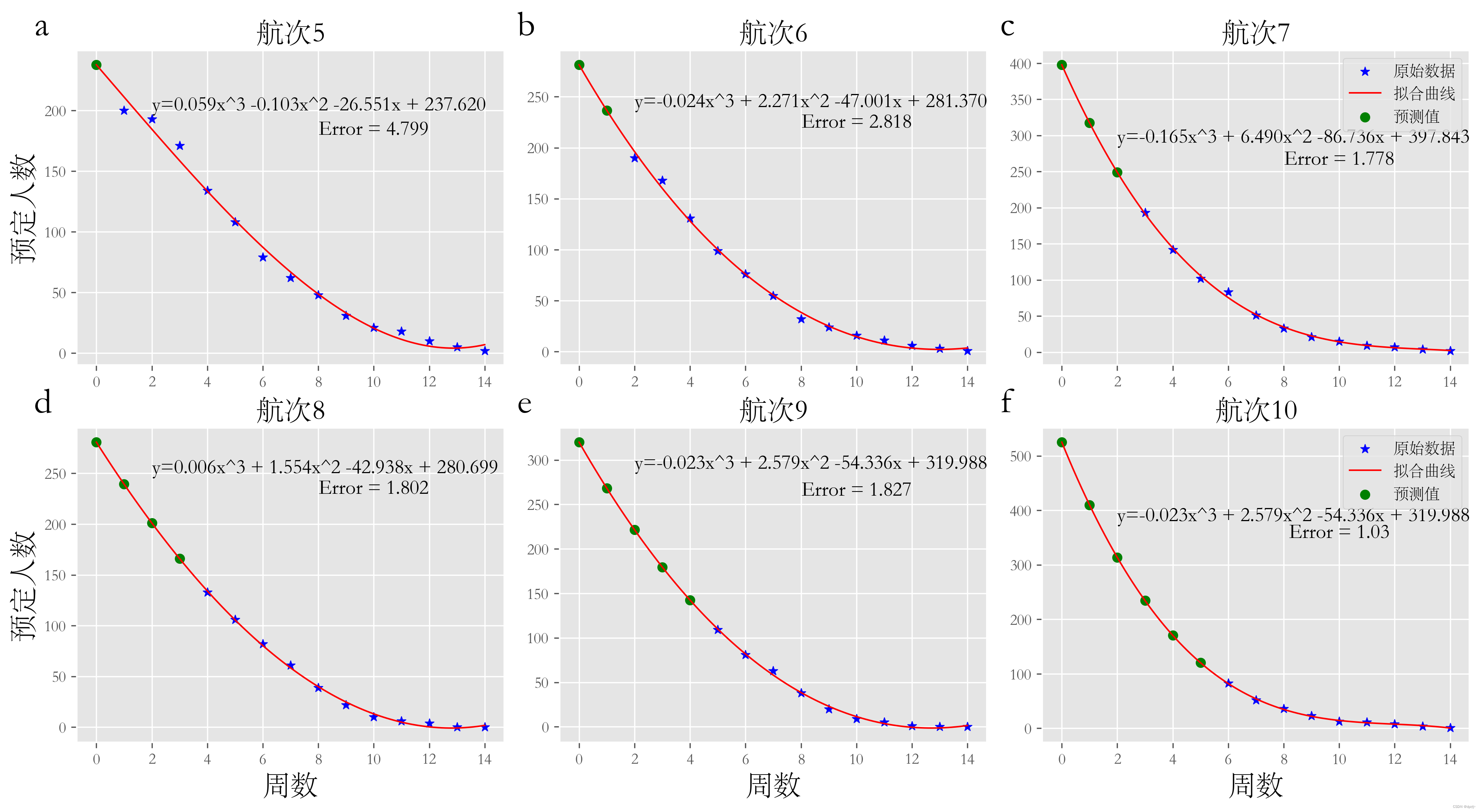
初学,写作灼虐,见谅!


 2288
2288


 被折叠的 条评论
为什么被折叠?
被折叠的 条评论
为什么被折叠?
 到【灌水乐园】发言


