深度学习——以天气识别为例，探讨如何保存神经网络模型

ysxAshore

已于 2022-08-08 20:07:28 修改

阅读量1.3k

点赞数 2

分类专栏： # 动手学深度学习——Pytorch 文章标签：神经网络 tensorflow keras cnn 图像处理

于 2022-08-08 15:23:12 首次发布

本文链接：https://blog.csdn.net/weixin_53966032/article/details/126223046

版权

动手学深度学习——Pytorch 专栏收录该内容

9 篇文章 4 订阅

订阅专栏

活动地址：CSDN21天学习挑战赛

如何保存神经网络模型

在训练时保存模型

ModelCheckpoint()函数的介绍

如何保存神经网络模型

在训练时保存模型

在训练时保存模型主要是利用 ModelCheckpoint() 函数的功能

ModelCheckpoint()函数的介绍

ModelCheckpoint()函数的全称是 tf.keras.callbacks.ModelCheckpoint

函数的主要功能是在指定的epoch后，保存模型到指定的路径处
def __init__(self,
               filepath,
               monitor='val_loss',
               verbose=0,
               save_best_only=False,
               save_weights_only=False,
               mode='auto',
               save_freq='epoch',
               options=None,
               initial_value_threshold=None,
               **kwargs):
filepath：str类型，保存模型的路径

当设置save_weights_only为False，即保存模型时，传的filepath需要是已存在的目录

当设置save_weights_only为True，即保存模型权重时，传的filepath需要是已存在的文件

monitor：dtr类型，表示监视值，可以是 val_accuracy、val_loss、accuracy和loss
verbose: 默认是0，表示输出不显示保存信息，为1表示显示信息,具体信息可见下图的Epoch 1：

save_best_only：默认为False，表示保存所有调用回调函数时的模型（可以选择加载最新的模型），如果为True，表示仅保存在验证集上表现最好的模型
save_weights_only：默认为False，表示是否仅保持模型的权重参数，为False是指表示整个模型

mode：str类型，可以是”auto“、"max"、"min" 三者之一，auto时较常用，可以由monitor值自动推断出mode值（accuracy——max，loss——min 包括val也是这样对应）

还可以传period参数，默认为1，表示隔1个epoch就进行函数回调

使用时，一般只需要传参 filepath、save_best_only和save_weights_only即可，其余参数视情况补充

保存模型权重参数

这里我们选择之前的MNIST手写数字识别所搭建的网络模型

(train_image, train_label), (test_image, test_label) = tf.keras.datasets.mnist.load_data()
train_image = train_image / 255.0
test_image = test_image / 255.0
train_image = train_image.reshape((-1, 28, 28, 1))
test_image = test_image.reshape((-1, 28, 28, 1))

model = models.Sequential([
    layers.Conv2D(32, (3, 3), padding="same", activation="relu", input_shape=(28, 28, 1)),
    layers.MaxPooling2D(),

    layers.Conv2D(64, (3, 3), activation="relu", padding="same"),
    layers.MaxPooling2D(),

    layers.Flatten(),
    layers.Dense(64, activation="relu"),
    layers.Dense(10)
])

model.summary()
model.compile(optimizer="adam",
              metrics="accuracy"
              , loss=tf.keras.losses.SparseCategoricalCrossentropy(from_logits=True))
history = model.fit(train_image, train_label, epochs=10, validation_data=(test_image, test_label))

# 输出网络模型loss、val_loss变化曲线
plt.plot(history.history['accuracy'], label='accuracy')  # 训练集准确度
plt.plot(history.history['val_accuracy'], label='val_accuracy ')  # 验证集准确度
plt.plot(history.history['loss'], label='loss')  # 训练集损失程度
plt.plot(history.history['val_loss'], label='val_loss')  # 验证集损失程度
plt.xlabel('Epoch')  # 训练轮数
plt.ylabel('value')  # 值
plt.ylim([0, 1.5])
plt.legend(loc='lower left')  # 图例位置
plt.show()

pre = model.predict(test_image)
plt.figure(figsize=(10, 20))
for i in range(10):
    print(np.array(pre[i]).argmax())
for i in range(10):
    plt.subplot(5, 10, i + 1)
    plt.xticks([])
    plt.yticks([])
    plt.grid(False)
    plt.imshow(test_image[i], cmap=plt.cm.binary)
    plt.xlabel(test_label[i])
plt.show()

保存模型参数主要包括以下几部分操作：

设置保存路径

# 设置路径地址
save_path = "net/weights/mnist.ckpt"
# 创建新文件 os.open(file_url,os.O_CREAT)
save_dir = os.path.dirname(save_path)
os.makedirs(save_dir)
os.open(save_path, os.O_CREAT)

# 也可以使用pathlib库创建

编写回调函数

cp_callback = tf.keras.callbacks.ModelCheckpoint(
    filepath=save_path,
    save_weights_only=True
)

fit添加回调函数并进行编译运行神经网络

model.fit(train_image, train_label, 
            epochs=10, 
            validation_data=(test_image, test_label),
            callbacks=[cp_callback])

保存的数据文件有：

使用保存好的模型参数（默认是加载最新的）：

# 读取保存好的模型参数
save_path = "net/weights/mnist/mnist.ckpt"
val_loss, val_accuracy = model.evaluate(test_image, test_label, verbose=1)
model.load_weights(save_path)
val_loss, val_accuracy = model.evaluate(test_image, test_label, verbose=1)

# 利用加载好的模型参数预测
pre = model.predict(test_image)
plt.figure(figsize=(10, 20))
for i in range(10):
    print(np.array(pre[i]).argmax())
for i in range(10):
    plt.subplot(5, 10, i + 1)
    plt.xticks([])
    plt.yticks([])
    plt.grid(False)
    plt.imshow(test_image[i], cmap=plt.cm.binary)
    plt.xlabel(test_label[i])
plt.show()

这是训练时的最后一次epoch的val_loss、val_accuracy

这是未加载参数时网络模型的 val_loss、val_accuracy

这桑加载完保存好的参数时网络模型的val_loss、val_accuracy

观察得到最后一次epoch时数据与加载后数据相一致

所以默认加载的是最后一次的epoch时的权重参数

保存整个网络

保存整个网络时，需要用到的路径需要是一个目录

回调函数处的 save_weights_only也需要改为False，至于save_best_only取决于用户需要（这里默认保存的是最后一次epoch时的模型，True是保存训练过程中，val_loss最低的模型）

保存模型的相关代码如下：
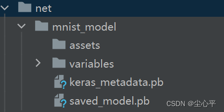
# 设置路径地址
save_path = "net/mnist_model"
# 创建目录
pathlib.Path.mkdir(pathlib.Path(save_path),parents=True)

cp_callback = tf.keras.callbacks.ModelCheckpoint(
    filepath=save_path,
    save_weights_only=False
)

model.fit(train_image, train_label, epochs=10, validation_data=(test_image, test_label),
          callbacks=[cp_callback])
保存整个模型的文件夹内的文件：

加载模型是通过 tf.keras.models.load_model() 加载，具体用法见后面的SavedModel方式介绍

SavedModel方式

使用SavedModel方式较为简单，主要是通过 model.save(路径) 保存模型和 tf.keras.models.load_model(路径) 加载模型，这里的路径也是目录

保存以后的目录内的文件也是下面的图片：

使用方法

model.save(目录路径)

model=tf.keras.models.load_model(目录路径)

示例代码

(train_image, train_label), (test_image, test_label) = tf.keras.datasets.mnist.load_data()
train_image = train_image / 255.0
test_image = test_image / 255.0
train_image = train_image.reshape((-1, 28, 28, 1))
test_image = test_image.reshape((-1, 28, 28, 1))

model = models.Sequential([
    layers.Conv2D(32, (3, 3), padding="same", activation="relu", input_shape=(28, 28, 1)),
    layers.MaxPooling2D(),

    layers.Conv2D(64, (3, 3), activation="relu", padding="same"),
    layers.MaxPooling2D(),

    layers.Flatten(),
    layers.Dense(64, activation="relu"),
    layers.Dense(10)
])

model.summary()
model.compile(optimizer="adam",
              metrics="accuracy"
              , loss=tf.keras.losses.SparseCategoricalCrossentropy(from_logits=True))
history = model.fit(train_image, train_label, epochs=10, validation_data=(test_image, test_label))

# 读取保存好的模型参数
save_path = "net/mnist_model"
model.save(save_path)
val_loss, val_accuracy = model.evaluate(test_image, test_label, verbose=1)
model1 = tf.keras.models.load_model(save_path)
val_loss, val_accuracy = model1.evaluate(test_image, test_label, verbose=1)
pre = model1.predict(test_image)
plt.figure(figsize=(10, 20))
for i in range(10):
    print(np.array(pre[i]).argmax())
for i in range(10):
    plt.subplot(5, 10, i + 1)
    plt.xticks([])
    plt.yticks([])
    plt.grid(False)
    plt.imshow(test_image[i], cmap=plt.cm.binary)
    plt.xlabel(test_label[i])
plt.show()

HDF5 格式

HDF5格式的使用与SavedModel的使用类似，主要是保存的路径不再是个目录而是个h5文件

仍是用model.save()、tf.keras.models.load_model() 两个方法

model.save(文件名.h5)

model=tf.keras.model.load_model(文件名.h5)

天气识别

数据集的下载

数据集可以在百度飞桨 Ai Studio 中搜索到

数据集链接天气识别数据集 - 飞桨AI Studio 下载解压即可

代码

具体操作已在代码中注释，针对过拟合，采用Dropout=0.4

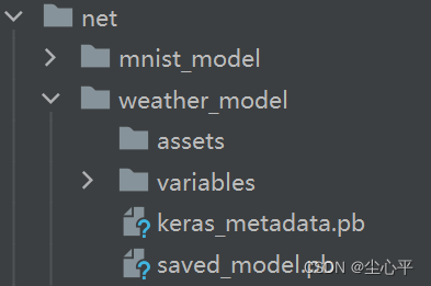
# 天气识别
# 设置本地数据集地址
data_url = "E:/Download/data_set/weather_photos"

# 指定标签名
class_names = ["cloudy", "rain", "shine", "sunrise"]
# 指定图像长宽
image_height = 256
image_width = 256
# 导入数据集
train_datas = keras.preprocessing.image.image_dataset_from_directory(
    directory=data_url,
    class_names=class_names,
    image_size=(image_height, image_width),
    seed=123,
    validation_split=0.2,
    subset="training",
    interpolation="lanczos3"
)
test_datas = keras.preprocessing.image.image_dataset_from_directory(
    directory=data_url,
    class_names=class_names,
    image_size=(image_height, image_width),
    seed=123,
    validation_split=0.2,
    subset="validation",
    interpolation="lanczos3"
)
train_datas = train_datas.cache().shuffle(500).prefetch(tf.data.AUTOTUNE)
test_datas = test_datas.cache().prefetch(tf.data.AUTOTUNE)
# 构建卷积神经网络
model = models.Sequential([
    layers.Rescaling(1 / 255.0, input_shape=(image_height, image_width, 3)),

    layers.Conv2D(32, (3, 3), padding="same", activation="relu", input_shape=(None, None, 3)),
    layers.MaxPooling2D(),

    layers.Conv2D(64, (3, 3), activation="relu", padding="same"),
    layers.MaxPooling2D(),

    layers.Conv2D(64, (3, 3), activation="relu", padding="same"),
    layers.MaxPooling2D(),

    layers.Flatten(),
    layers.Dropout(0.4),
    layers.Dense(64, activation="relu"),
    layers.Dense(4)
])
model.summary()

# 编译训练网络模型
model.compile(optimizer="adam",
              loss=tf.keras.losses.SparseCategoricalCrossentropy(from_logits=True),
              metrics=['accuracy'])
# 在model.fit 
history = model.fit(train_datas, validation_data=test_datas, epochs=10)

# 输出网络模型loss、val_loss变化曲线
plt.plot(history.history['accuracy'], label='accuracy')  # 训练集准确度
plt.plot(history.history['val_accuracy'], label='val_accuracy ')  # 验证集准确度
plt.plot(history.history['loss'], label='loss')  # 训练集损失程度
plt.plot(history.history['val_loss'], label='val_loss')  # 验证集损失程度
plt.xlabel('Epoch')  # 训练轮数
plt.ylabel('value')  # 值
plt.ylim([0, 1.5])
plt.legend(loc='lower left')  # 图例位置
plt.show()


# 预测
pre = model.predict(test_datas)
for i in range(20):
    print(pre[i])
    print(class_names[numpy.array(pre[i]).argmax()])
# 绘画数据集图像，查看导入是否完成
plt.figure(figsize=(20, 10))
for test_image, test_label in test_datas.take(1):
    for i in range(20):
        plt.subplot(5, 10, i + 1)
        plt.xticks([])
        plt.yticks([])
        plt.grid(False)
        plt.imshow(test_image[i].numpy().astype('uint8') / 255.0, cmap=plt.cm.binary)
        plt.xlabel(class_names[test_label[i]])
    plt.show()

# 用savedmodel方式保存整个网络，也可以用.h5文件，也可以用checkpoint保存整个模型
# 也可以用checkpoint保存权重参数加载模型
save_path = "net/weather_model"
model.save(save_path)

保存的目录结构

加载所保存的模型，进行预测

save_path = "net/weather_model"
model = tf.keras.models.load_model(save_path)
pre = model.predict(test_datas)
for i in range(32, 42):  # batch_size 默认为32
    print(pre[i])
for i in range(32, 42):  # batch_size 默认为32
    print(class_names[numpy.array(pre[i]).argmax()])

for test_image, test_label in test_datas.take(2):
    for i in range(20): # 第二张图前十个天气是预测的真实值
        plt.subplot(5, 10, i + 1)
        plt.xticks([])
        plt.yticks([])
        plt.grid(False)
        plt.imshow(test_image[i].numpy().astype('uint8') / 255.0, cmap=plt.cm.binary)
        plt.xlabel(class_names[test_label[i]])
    plt.show()

真实值：

预测值：

[-20.913506 -13.227225  -6.835453  16.999655]
[  3.6401439    3.7265291    0.96968377 -10.230032  ]
[  2.0867512   4.413174    0.4877592 -10.106009 ]
[-5.611314  -6.928367   1.4171107  2.662863 ]
[ 4.0711594 -4.901644   3.7610795 -6.6193724]
[ 1.510512    6.4153357  -0.17131034 -9.647087  ]
[ 5.199197  -1.9983941 -2.0065382 -3.3040116]
[ 0.04972115 -3.3614075   4.4348345  -8.757731  ]
[ 0.49389228  5.2676754  -0.5260849  -8.89126   ]
[-1.826133  -5.6637144  3.5098753 -6.234786 ]
sunrise
rain
rain
sunrise
cloudy
rain
cloudy
shine
rain
shine

ysxAshore

关注

2
点赞
踩
7

收藏

觉得还不错? 一键收藏
0
评论
深度学习——以天气识别为例，探讨如何保存神经网络模型

本篇博客主要是总结神经网络模型的保存方法，具体总结了SaveModel、HDF5和Checkpoint三种方法（其中的checkpoint除保存整个模型外还可以保存权重信息），最后博客以天气识别的示例进行了保存神经网络模型的演练...
复制链接

扫一扫