


本篇介绍基础包stats中的一个函数nls(),它的作用是求解非线性回归的待定参数。
nls(formula, data, start,
    control, algorithm,
    trace, subset, weights,
    na.action, model,
    lower, upper, ...)
主要参数的要求如下:
formula:非线性回归的形式,格式为
y ~ f(x1, x2,...);data:数据源;一般为数据框或列表结构,不能为矩阵结构;
start:待定参数的起始值;列表结构。
比如,S型曲线可以很好地拟合传染病感染人数的增加趋势。本文示例使用的数据是2020年1月至3月我国新冠肺炎的确诊人数(示例数据可在后台发送关键词“示例数据”获取)。
library(readxl)
covid <- read_xlsx("107.1-china-covid19.xlsx",sheet = 1)

library(tidyverse)
library(magrittr)
data <- covid %>%
  group_by(date) %>%
  summarise(total = sum(confirmed))
plot(data$total, type = "l")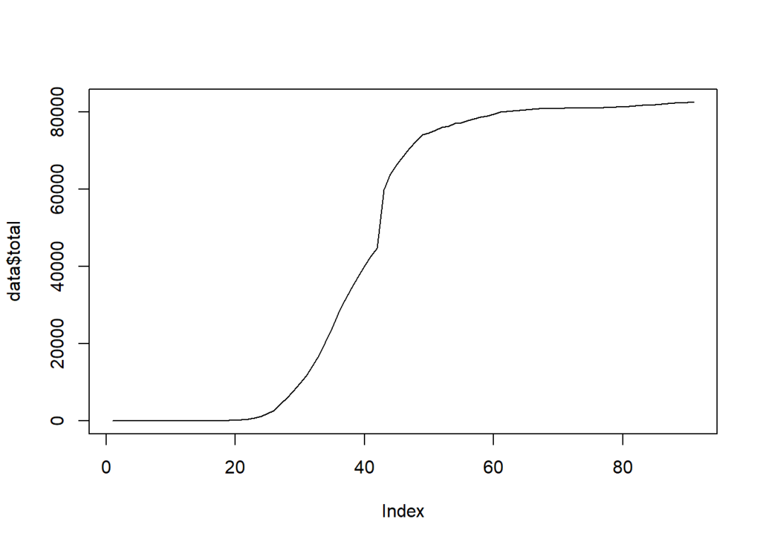
从上图可以看出,累积确诊人数的增长趋势大致呈S型。
一个典型的S型曲线的函数形式如下:
Scurve = function(t, a, b, c)
  return(c/(1+exp(a*t+b)))

v = apply(matrix(-10:10), 1, Scurve,
      a = -1, b = 0, c = 80000)
plot(-10:10, v, type = "l")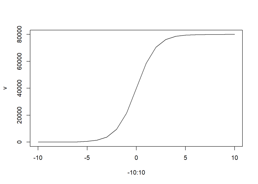
下面使用nls()函数求解S型函数的相关参数,也就是a、b、c。
data$t = 1:dim(data)[1]
fit <- nls(formula = total ~ Scurve(t, a, b, c),
           data = data,
           start = list(a = -1, b = 10, c = 80000))
fit
## Nonlinear regression model
##   model: total ~ Scurve(t, a, b, c)
##    data: data
##          a          b          c
##    -0.2225     8.7560 81216.6896
##  residual sum-of-squares: 202669699
##
## Number of iterations to convergence: 8
## Achieved convergence tolerance: 9.394e-06
需要注意的是,起始值的选择非常关键,要尽量靠近真实值,若相差太大可能会报错。
plot(data$t, data$total, type = "l",
     xlab = "天数", ylab = "累积确诊数")
lines(fitted(fit), col = "red",
      lty = 2)
legend("topleft", legend = c("原始数据", "拟合值"),
       lty = c(1,2), col = c("black", "red"))
下面仅使用前50天的数据来拟合S型曲线。
data2 = data[1:50,]
fit2 <- nls(formula = total ~Scurve(t, a, b, c),
            data = data2,
            start = list(a = -1, b = 10, c = 80000))
fit2
## Nonlinear regression model
##   model: total ~ Scurve(t, a, b, c)
##    data: data2
##          a          b          c
##    -0.2105     8.4264 86016.4864
##  residual sum-of-squares: 159722376
##
## Number of iterations to convergence: 16
## Achieved convergence tolerance: 8.084e-06

plot(data2$t, data2$total, type = "l",
     xlab = "天数", ylab = "累积确诊数",
     xlim = c(1,91), ylim = c(0, 85000))
lines(predict(fit2, data), col = "red",
      lty = 2)
legend("topleft", legend = c("原始数据", "拟合值"),
       lty = c(1,2), col = c("black", "red"))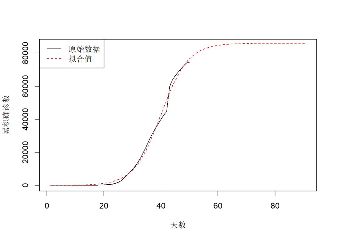


 被折叠的 条评论
为什么被折叠?
被折叠的 条评论
为什么被折叠?
 到【灌水乐园】发言


