Python极简讲义一本书入门机器学习和数据分析--自学笔记

0 前言

本书有的知识点之前说，过了几节后再解释。有几个错误但是影响不大。作者自己找补说，有的没讲正常，主要靠自学。
我这里对一些没讲的作了一些补充。
这里是这本书和源码的百度链接，分享给大家。
链接： https://pan.baidu.com/s/1d4-gC7kzRvIxilWmbayrSg?pwd=ciav
提取码：ciav
还不完善: 有几章的题还没写.

1 初识python和jupyter

MAKE

最小必要知识(MAKE),迅速掌握MAKE,然后缺啥补啥.

jupyter

jupyter脱胎于ipython项目。ipython是一个python交互式shell，它比默认的python shell 要好用很多。而ipython正式jupyter的内核所在，我们可以理解为，jupyter是网页版的ipython。
esc 退出编辑模式
d d删除 l 显示行数 a 向上增加行 b 向下增加行

魔法函数

jupyter的魔法函数，脱离ipython的使用环境，如pycharm是用不了的。
魔法函数分为面向行和面向块的。
%matplotlib inline 内嵌
%matplotlib qt 单独
想知道用法直接%timeit? 最后追加问号
%%timeit针对代码块 两个百分号是针对整个代码块的
建议 把测试运行时长单独放置一个单元格中
%%writefile name.py 对代码块生产 .py文件

2 结构类型与程序控制结构

. 调用的是方法
不用 . 调用是内置函数

基本数据类型

数值

布尔

and 优先级比 or 高 会先运算
复数a+bj
type()只能输出一个变量的类型
多个变量同时赋值 a, b, c = 1, 0.5, 1+1j

字符串

方框调用
split(" ")依据空格分片为列表
title() 首字母大写其余小写

str1 = "i love you beijing"
str1.split(" ")
# ['i', 'love', 'you', 'beijing']

strip(‘abc’)删除字符串两端的abc 默认空格
字符串前缀

• b 后面字符串是bytes类型 网络编程中,只认bytes
• u/U 表示unicode字符串
• r/R 非转义的原始字符串,去掉反斜杠的转义机制

格式化输出

• %s格式化 ：和c语言类似

print ("我叫 %s 今年 %d 岁!" % ('小明', 10))
# 我叫 小明 今年 10 岁!

• format格式化
  {}内填

"{},{}".format("hello","world")
"{1},{0}".format("hello","world")
"{0},{1},{0},{0}".format("hello","world")
print("{:.2f}".format(3.1415926))

• f-string格式化
• f-string 格式化字符串以 f 开头，后面跟着字符串，字符串中的表达式用大括号 {} 包起来，它会将变量或表达式计算后的值替换进去
• {} 相当于c语言的百分号

print(f'hello world {str1}')
# hello world i love you beijing

大括号内外不能用同一种引号，需根据情况灵活切换使用单引号、双引号、单三引号、双三引号。
大括号内不能使用 \ 转义
需要显示大括号，则应输入连续两个大括号{{ }}；大括号内需要引号，使用引号即可。

print(f'i am {"hua wei"}')
print(f'{{5}}{"apples"}')

填充

冒号后写数据格式
记忆方法：括号口朝左边，就表示左填充；括号口朝右边，就表示右填充

print(f'{1:0>4}')
# 输出4个字符，不足补0
# 0001

数字符号相关格式描述符：仅针对数值有效

• + 正负数都输出符号
• - 负数输出符号
• 空格 正数加空格 负数加负号
• width.precision

print(f'{1:+}')
#+1
print(f'{1: }\n{-1: }')
# 1
#-1
a = 123.456
print(f"{a:.2f}")
#123.46

列表

反向索引 -i 表示倒数第 i 个元素 例如-1表示倒数第一个元素，但是0表示第一个元素，要注意。
list[0:5],左闭右开，取前五个元素l ist1[::2] 步长为2
list1[::-1]步长为-1，即为倒着输出
访问单个元素注意返回的不是列表.

testlist = [1,3,3,677]
print(type(testlist[0]),type(testlist[1:3]))
#<class 'int'> <class 'list'>

+ 连接列表, * 整体复制列表

a = [1, 2, 3]
b = [4, 5, 6]
a + b # 连接[1, 2, 3, 4, 5, 6]
a * 3 # 整体复制3次[1, 2, 3, 1, 2, 3, 1, 2, 3]

list() 将字符串等可迭代对象转化成列表

list_ = list("hello world")
print(list_)
# ['h', 'e', 'l', 'l', 'o', ' ', 'w', 'o', 'r', 'l', 'd']

添加列表元素

• append(): 在列表尾部添加一个新元素
• insert():在指定索引位置插入一个元素
• extend():把一个列表整体添加到另一个列表的尾部

a.append(9)
a.insert(2,0) 
# 在2号位插入数字0
a.extend(b)

id(a)返回a的地址
删除列表元素

id(a)
# 2932207713216

• pop():默认删除尾部一个元素，或者删除指定索引元素
• remove(x):删除第一个与x相同的元素
• clear():清空列表所有元素

stlist.pop()
stlist.pop(3)
stlist.remove('a')
stlist.clear()

del 删除到变量到对象的引用和变量名称本身
注意del语句作用在变量上，而不是数据对象上

del stlist[:2]
# 删除前2个元素

• count(x)：x出现的个数
• index(x)：x首次出现的位置
• in / not in ：是否存在

slist.count(1)
slist.index(2)
if 5 not in slist:
    print("hello")
else:
    print("aloha")

列表元素排序

• sort() ：按字典顺序排序
  当元素之间的类型不能够互相转换的时候，Python就会报错，例如整数和字符串类型
• reverse() ：倒置

fruits.sort()
print(fruits)
fruits.reverse()
print(fruits)
print(fruits[::-1])
# 也可以逆序

• sort(key = None, reverse = false): key是指定比较的元素，reverse 为 True则逆序，默认顺序。
• sorted(iterable, key=None, reverse=False) ：全局内置函数 复制原始列表的一个副本，再排序。而sort()会改变数据。

fruits.sort(cmp = None, key = None, reverse = True)
sorted(fruits,reverse = True)

其他全局内置函数

• cmp(),不可用 operator模块的函数替代之
• len() ：元素个数
• max(),min() ：最大最小值
• list() ：转换成列表
• range(start, stop[, step])返回整数序列的对象，而不是列表
• zip()：用于将可迭代的对象作为参数，将对象中对应的元素打包成一个个元组，然后返回对象，而不是列表。如果各个迭代器的元素个数不一致，则返回列表长度与最短的对象相同，如果只有一个可迭代对象,那么zip()会找到空元素来代替.
  利用 * 号操作符，可以将可迭代对象解包。
• enumerate(sequence, [start=0])：用于将一个可遍历的数据对象(如列表、元组或字符串)组合为一个索引序列(索引, 元素)，同时列出数据和数据下标，一般用在 for 循环当中。
• zip()可以完成多个类型的缝合，而enumerate只能提供数值类型

import operator
operator.lt(1,2)
# 是否小于
list(zip(fruits,range(len(fruits))))

'''
[('apple', 0),
 ('banana', 1),
 ('orange', 2),
 ('watermelon', 3),
 ('apple', 4),
 ('blueberry', 5),
 ('strawberry', 6)]
'''
list(zip(*zip(fruits,range(len(fruits)))))
'''
[('apple',
  'banana',
  'orange',
  'watermelon',
  'apple',
  'blueberry',
  'strawberry'),
 (0, 1, 2, 3, 4, 5, 6)]
'''
list(enumerate(fruits,start = 1) )
'''
[(1, 'apple'),
 (2, 'banana'),
 (3, 'orange'),
 (4, 'watermelon'),
 (5, 'apple'),
 (6, 'blueberry'),
 (7, 'strawberry')]
'''
for i,ele in enumerate(fruits,start = 1):
    print(i,ele)
'''
1 apple
2 banana
3 orange
4 watermelon
5 apple
6 blueberry
7 strawberry
'''

元组

一旦创建便不能修改
如果只有一个元素必须加逗号，必不可少，逗号是一个元组的核心标识
操作与列表类似
tuple()将字符串，列表等可迭代对象转化为元组

tuple("hello world")
# ('h', 'e', 'l', 'l', 'o', ' ', 'w', 'o', 'r', 'l', 'd')
a = (1,2,3)
b = (4,5,6)
c = a + b
print(c)
# (1, 2, 3, 4, 5, 6)

实在想要修改的话

c = c[:2] + (7,) + c[2:]
# 但是此时c已经不是之前的c了

字典

键值对，键必须要独一无二
列表无法作为字典的键
字典无法作为字典的键或集合的元素

• items()：显示所有键值对，一一封装在元组里
• keys()：显示键
• values()：显示值

dict1 = {'a':1,'2020':[1,2,3],100:('hello','world')}
dict1.items()
# dict_items([('a', 1), ('2020', [1, 2, 3]), (100, ('hello', 'world'))])
dict1.keys()
dict1.values()

输出某个键对应的值

• dict1[x] x是键的名字

dict1[100]
# ('hello','world')

get(key,default = None)方法

dict1.get('b','无此键')
# '无此键'

字典可变，修改直接赋值即可
增加元素，直接用方括号给出新键并赋值即可

dict1[(1,2)] = "asljdlas"
# {'a': 2, '2020': [1, 2, 3], 100: ('hello', 'world'), (1, 2): 'asljdlas'}

将一个字典整体增加到另一个字典

• update(x) ：相当于列表或者元组的 +

t1 = {'asd':[1,2],(1,2):'s'}
dict1.update(t1)
# {'a': 2, '2020': [1, 2, 3], 100: ('hello', 'world'), (1, 2): 's', 'asd': [1, 2]}

• pop(x) ：删除键为 x 的字典元素
• popitem()：删除字典最后一个元素

dict1.pop(100)
dict1.popitem()
# {'a': 2, '2020': [1, 2, 3], (1, 2): 's'}

集合

{}围住，无序，唯一
集合元素只能包括数值，字符串，元组等不可变元素
不能包括列表，字典和集合等可变元素
即使强制重复也会自动去重

set1 = {1,2,2,3,3}
# {1, 2, 3}

• set() 将可迭代对象转换为集合

可以用 | & - ^ 求两个集合的并，交，差，对称差
也可以用方法

程序控制结构

python中的数值型非0为真，None、空字符串、空列表、空元组、空字典、空集合都是false。

选择

if else
if elif…
if else 三元操作符

x = 10
y = 20
small = x if x < y else y
print(small)

循环

对字典d 可以迭代键，不能迭代k，v
或者k,v解包 items()

for k in d():
	print(k,d[k])
	# 或者 print(k,d.get(k,0))
for k,v in d.items():
    print(k,v)

number = [1,55,123,-1,44,77,8]
even = []
odd = []
while len(number) > 0:
    a = number.pop()
    if a % 2 == 1:
        even.append(a)
    else:
        odd.append(a)
print(f'even: {even}\nodd: {odd}')
'''
even: [77, -1, 123, 55, 1]
odd: [8, 44]
'''

推导式

[生成表达式 for 变量 in 序列或迭代对象]

列表推导式

alist = [x**2 for x in range(1,11)]

过滤不符合条件的元素

int_list = [x for x in a if type(x) == int]

for循环可以嵌套 也可以用多条for if构建

字典推导式

dic = {1:'a',2:'b',3:'c'}
reverse_dic = {v:k for k, v in dic.items()}
# {'a': 1, 'b': 2, 'c': 3}

集合推导式

sq = {x**2 for x in [1,-1,2,2,3]}
# {1, 4, 9}

例题

list1 = [1,2,3]
list2 = [2,7]
liste = []
for i in list1:
    for j in list2:
        if i != j:
#             t = [i,j]
            liste.append((i,j))
# 或者
difflist = [(a,b) for a in list1 for b in list2 if a != b]

3.删除列表中的重复元素

• set()最方便

duplist = [1,1,2,2,4,'a','b','a',3,1]
list3 = list(set(duplist))

• 利用字典的键

dict4 = {}
for i in duplist:
    dict4[i] = 1
list5 = list(dict4.keys())
print(type(dict4.keys()),type(list(dict4.keys())))
# <class 'dict_keys'> <class 'list'>
# 注意keys()方法不是列表类型
print(list5)

4.删除小于3个字符的姓名 ,相同的名字合并

names = ['alice','bob','Bob','Alice','J','JOHN','Bob']
# uni_names = {i.title() for i in names if len(i) > 2}
uni_names = {name[0].upper() + name[1:].lower() for name in names if len(name) > 2}
# 花括号是集合
print(uni_names)

5 键不分大小写，将值合并

mcase = {'a':10, 'b':34, 'A':7, 'Z':3}
fcase = {key.lower():mcase.get(key.upper(),0) + mcase.get(key.lower(), 0) for key in mcase.keys()}
# {'a': 17, 'b': 34, 'z': 3}
# 

# 法二
f2case = {}
for key in mcase.keys():
    f2case[key.lower()] = mcase.get(key.lower(),0) + mcase.get(key.upper(), 0)
    # 没有则返回0
    #     f2case[key.lower()] = mcase[key.lower()] + mcase[key.upper()]
    # 直接读取不存在的键会报错

注：upper和lower是字符串的方法
get是字典的方法
keys()整体是dict_keys类型，每个键的类型各有不同。

3 自建Python模块与第三方模块

导入Python标准库

import 模块名 as 别名
from 模块名 import 对象名 as 别名
模块名.函数名
别名.函数名
导入某个特定对象后 可以直接使用函数 全局变量等

编写自己的模块

一个.py文件就可以称为一个模块。
假设当前模块声明了这个内置变量,如果本模块直接执行,那么这个__name__的值就为__main__.
如果它被第三方引用(即通过import导入),那么它的值就是这个模块名,即它所在python文件的文件名.

__name__ 为模块名

parameters模块

PI = 3.1415926
def paraTest():
    print('PI = ',PI)

if __name__ == '__main__' :
    paraTest()

from parameters import PI
def circleArea(radius):
    return radius ** 2 * PI
def run(radius):
    print('圆的面积为: ',circleArea(radius))
run(5)

import sys
sys.path

包(Package)

模块一般就是我们日常随手用的一些规模较小的代码，而在比较大规模的任务一般需要用到大量的模块，此时我们可以使用包(Package)来管理这些模块。我们平时下载的第三方包也就是这个，如Numpy,
2.1 什么是包？包，就是里面装了一个__init__.py文件的文件夹。init.py脚本有下列性质：（1）它本身是一个模块；（2）模块名不是__init__，而是包的名字，也就是装着__init__.py文件的文件夹名。（3）它的作用是将一个文件夹变为一个Python模块（4）它可以不包含代码，不过一般会包含一些Python初始化代码(例如批量导入需要的模块)，在这个包被import的时候，这些代码会自动被执行。
导入包的方法和导入模块比较类似，只不过由于层级比一般模块多了一级，所以多了一条导入形式.
import 包名.模块名import 包名.模块名 as 模块别名

常用的内建模块

collections模块

namedtuple

第二个参数 [“x”,“y”]也可以写成 “x y"或者"x,y”
变量名不一定要和第一个参数相同
不同属性用逗号隔开，用属性来访问命名元组中的某个元素。

from collections import namedtuple
Point = namedtuple('Point',['x','y'])
p = Point(3, 4)
print(p.x, p.y)
#3 4
p = p._replace(x = 5)
# p[0] 第一个元素 索引调用完全可以
# 修改需要调用_replace方法

x,y = p
# 解包 把一个包含多个元素的对象赋给多个变量

deque 双向队列

和list形式上很像，都是方括号，但是list的写操作当列表元素数据量很大时，效率低。
没有sort方法。

• append 右边增加元素
• appendleft 左边增加元素
• pop 弹出最右边元素
• popleft 弹出最左边元素
• insert(index,x)插入到index号 元素为x
• remove(x) 移除第一个为x的元素
• reverse 颠倒
• rotate(x) 循环整体向右移动x位
• extend(iterable)可迭代对象添加到尾部
• 字符串也是可迭代对象，如直接添加字符串’ABC’，会将’A’、‘B’、'C’添加到队列中
• extendleft 添加到首部
• copy 列表元组都有此方法
• count
• index
• maxlen
• 指定队列的长度后，如果队列已经达到最大长度，此时从队尾添加数据，则队头的数据会自动出队。队头的数据相等于被队尾新加的数据“挤”出了队列，以保证队列的长度不超过指定的最大长度。反之，从队头添加数据，则队尾的数据会自动出队。

dq.extend('qbc')
# deque(['a', 'aa', 'c', 'b', 'x', 'abc', 'q', 'b', 'c'])

mdq = deque(maxlen = 5)
mdq.extend(['a','b','c','d','e','f'])
# deque(['b', 'c', 'd', 'e', 'f'], maxlen=5)

OrderedDict

有序字典，底层双向链表
update()
move_to_end(x)将键为x的元素移到尾部

defaultdict

dd = defaultdict(lambda : 'N/A')
dd['a'] ='china'
dd['c']
dd['z']
# {'a': 'china', 'c': 'N/A', 'z': 'N/A', 'b': 'N/A'}

Counter

统计每个单词出现的次数

colors = ['red','yellow','blue','red','black','red','yellow']
dict1 = {}
for _ in colors:
    if dict1.get(_) == None:
        dict1[_] = 1
    else:
        dict1[_] += 1
print(dict1)

dict2 = Counter(colors)
print(dict(dict2))

• most_common(n)求出现频率最高的n个单词

print(dict2.most_common(1)) # 出现频率最高的1个单词

datetime模块

一个模块可以有很多类

datetime模块的datetime类

from datetime import datetime

获取当前时间日期

datetime.now()

利用datetime构造方法生成时间

date1 = datetime(21,1,5)
print(date1,type(date1))
date1.day
# 0021-01-05 00:00:00 <class 'datetime.datetime'>
# >>> 5

纪元时间
1970年1月1日00:00:00 UTC+00:00 在计算机里记为0.
当前时间就是相对于纪元时间流逝的秒数，称为timestamp

时间日期调用timestamp()方法

datetime.now().timestamp()

将字符串转换为datetime
strptime方法
datetime.strptime(‘日期时间’,‘格式’)

cday = datetime.strptime('2023 4 16 Sun 11:30:00','%Y %m %d %a %H:%M:%S')
print(cday)
# 2023-04-16 11:30:00

%Y 四个数字表示的年份 %y 两个数字表示的年份
%m 月份
%M 分钟数
%H 24小时 %I 12小时
%d 天
%S 秒
%a 星期缩写 %A 星期全写
%b 月份缩写 %B 月份全写

将datetime转换为字符串
对象.strftime(格式)

date1 = now.strftime('%Y%m%d %a')
print(date1)
# 20230416 Sun

datetime加减
引入timedelta时间差类,参数英文要加s.

date2 = cday - timedelta(days = 2, hours = 12)
print(date2)
# 2023-04-13 23:30:00

求两个日期相差的天数
两个datetime变量相减自动成为timedelta类型

list1 = ['2023 4 16','2022-1-1']
lday1 = datetime.strptime(list1[0],'%Y %m %d')
lday2 = datetime.strptime(list1[1],'%Y-%m-%d')
deltadays = lday1 - lday2
print(type(deltadays))
print(deltadays)
# <class 'datetime.timedelta'>
# 470 days, 0:00:00

json模块

JSON书写格式类似于字典

• json.dumps() 将python序列化为JSON格式字符串
• json.loads() 将JSON格式字符串反序列化为python对象

random模块

• random() 同名方法,生成0-1之间的随机数 范围[0,1)
• uniform(x,y)生成[x,y]之内的随机数
• seed(n) 设置随机数种子,后续每次生成随机数都是相同的
• randoint(x,y)生成x,y之内的整型数
• randrange(start,end,step) 就是从range(start,end,step)中随机选一个
• choice(x)从x(列表,元祖,字典)中随便选一个
• choices(it, y)从it中选取多个,放回采样
• sample(it,y)从it中选取多个,不重复
• shuffle(x)打乱原有排序

random.seed(10)
random.random()

4 Python函数

Python中的函数

函数返回多个值

实际上函数返回的是一个元组的引用

def increase(x,y):
    x += 1
    y += 1
    return x,y
a,b = increase(1,2)
print(type(increase(1,2)));
'''
(2, 3)
<class 'tuple'>
'''

return [a,b]
# 也可以输出列表

函数文档

'''
一个问号看文档 两个问号看代码
help(函数名)
函数名.__doc__
'''
increase?? 
'''
Signature: increase(x, y)
Source:   
def increase(x,y):
    '''
    功能,对输入的两个数字自增1 并返回增加后的数
    '''
    x += 1
    y += 1
    return x,y
File:      c:\users\2021\appdata\local\temp\ipykernel_10168\799339069.py
Type:      function
'''
help(increase)
'''
Help on function increase in module __main__:

increase(x, y)
    功能,对输入的两个数字自增1 并返回增加后的数
'''
increase.__doc__
'''
'\n    功能,对输入的两个数字自增1 并返回增加后的数\n    '
'''

函数参数的花式传递

关键字参数

指定参数

参数为 word = 'hello world'

可变参数

在形参前面加* ,不管实参有多少个,在内部它们都存放在以形参名为标识符的元组中

*args

def varPara(num,*str):
    print(num)
    print(str)
varPara(5,'das','sadasd')
'''
5
('das', 'sadasd')
'''

可变参数例子

def mySum(*args):
    sum = 0
    for i in range(len(args)):
        sum += args[i]
    return sum
print(mySum(1,3,5,1.0 + 1j))
print(mySum(1.2,1.2,6.6))
# (10+1j)
# 9.0

可变关键字参数

两个星号

**kwargs

会把可变参数打包成字典
调用函数需要采用arg1 = value1,arg2 = value2的形式

def varFun(**args):
    if len(args) == 0:
#         print('None')
        return 'None'
    else :
#         print(args)
        return args
print(varFun())
print(varFun(a = 1,b = 2))
print(varFun(1,2))
'''
None
{'a': 1, 'b': 2}

---------------------------------------------------------------------------
TypeError                                 Traceback (most recent call last)
~\AppData\Local\Temp\ipykernel_14840\2103809882.py in <module>
      1 print(varFun())
      2 print(varFun(a = 1,b = 2))
----> 3 print(varFun(1,2))

TypeError: varFun() takes 0 positional arguments but 2 were given
'''

除了用等号给可变关键字参数赋值,还可以直接用字典给可变关键字参数赋值

默认参数

设定一个默认值,有就覆盖,没有就用默认的
如果列表L作为默认参数,列表是一个可变量,每次调用函数时,如果改变了L的内容,则下次调用时,默认参数就会改变,不再是函数刚开始定义时的那个空列表了.
定义默认参数的时候务必让这个默认参数是不可变对象,例如数值,元组,字符串,不可变集合(frozenset),None等

def add_end(L = None):
    if L is None:
        L = []
    L.append('END')
    return L

参数序列的打包与解包

打包:多个变量赋值给一个,会被打包成一个元组
解包:将一个可迭代对象元素分别赋值给分散对象

在可迭代对象前加一个*号,就可以解包了
对字典加一个星号,只能解包键(输出形参)
加二个星号,就可以正常解包了(输出values)

def fun(a,b,c,d):
    print(a,b,c,d)
list1 = [1,2,3,4]
fun(*list1)
dict1 = {'a':1,'x':2,'y':3,'d':4}
fun(*dict1)
# a x y d
fun(**dict1)
# 1 2 3 4

传值还是传引用

python中所有的函数参数传递,统统都是基于传递对象的引用进行的.这是因为,在python中,一切皆对象.而传对象,实质上传的是对象的内存地址,而地址即引用.
对象大致分为两大类,可变和不可变对象.可变包括字典,列表及集合等.不可变对象包括数值,字符串,元组等.
可变对象,传递的就是地址.就不需要return一个可变对象了.
不可变对象,为了维护它的不可变属性,函数不得不重构一个实参的副本,相当于值传递.

函数的递归

def recursive_fact(n):
    if n <= 1:
        return 1
    return n * recursive_fact(n - 1)
num = 5
result = recursive_fact(num)
print(f'递归方法: {num}! = {result}')

函数式编程的高阶函数

函数也是对象,因此函数(对象)可以作为参数,也可以返回一个函数(对象)

lambda表达式

只有一行代码的函数,由于其太过短小,用后即焚,不值得起名字
lambda 参数:对参数实施的操作
可以把lambda表达式赋值给一个变量,由于赋值可以决定被赋值对象的类型,所以这个变量在本质上也是一个函数,当我们使用这个变量时,实际上就是在调用lambda表达式.也就是说,上述操作,让一个原本匿名的函数变得"有名"了.

new_add = lambda x,y:x+y
print(new_add(3.2,1+5j),type(new_add))
# (4.2+5j) <class 'function'>

filter()函数

filter(function,iterable)
两个参数,第一个为判断函数,用于制定筛选规则,第二个为序列,作为第一个参数的数据.
序列中每个元素都将作为参数传递给函数进行判断,符合条件的(即判定为True的)留下,否则就淘汰出局

def fun(var):
    letters = list('aeiou')
    if var in letters:
        return True
    else:
        return False

sequence = list('sadasdwecsadisd')
filtered = filter(fun,sequence)
print(list(set(filtered)))
# ['i', 'a', 'e']

如果第一个函数参数功能非常简单,可以使用lambda表达式来描述

a_list  = [1,34,12,54,136,314,212,13,22,9]
print(list(filter(lambda x: x % 3 == 0,a_list)))
# [12, 54, 9]

map()函数

map(function, iterable, …)
参数：
function是映射函数
iterable是一个或多个可迭代序列
返回值：
迭代器
在第一个参数代表的函数加工下，第二个参数代表的数据源就会转换成一个新的序列

# 求字符串组成的列表的每个字符串的长度序列
def lenstr(n):
    return len(n)
list2  = list(map(lenstr,['hello','sad','byebye','china']))
print(list2)
#[5, 3, 6, 5]

# lambda改写
list3 = list(map(lambda x:len(x),('asd','qwewqeq','12334','xzcx')))
print(list3)

def myFunc(x,y):
    return x + y
# str_cat = map(myFunc,('1','ss','wxs'),('2','sda','wwww'))
str_cat = map(lambda x,y:x+y,('1','ss','wxs'),('2','sda','wwww'))
print(list(str_cat))
# ['12', 'sssda', 'wxswwww']

注:使用列表推导式也能完成类似功能.但是map()函数的出现,使得效率高很多.

reduce()函数

reduce的本意就是规约或减少
reduce(function,iterable,[,initializer])
function 实现规约功能的二元函数
iterable 可迭代对象
initializer 初试参数

reduce对一个可迭代对象中的所有数据执行下列操作,取前两个参数,利用function代表的规则进行计算,得到的结果再与iterable的第三个数据拼成一堆,然后再利用function代表的规则进行运算.得到下一个结果…以此类推.直到计算出最后一个结果.
reduce函数在python3的内建函数移除了，放入了functools模块

print((reduce(lambda x,y:x+y,range(101))))
# 5050

利用reduce函数求最大最小值

a_list = [1,5,234,888,2,1,0]
reduce(lambda x,y:x if x > y else y,a_list)
# 888

sorted()函数

sorted(iterable, key=None, reverse=False)
如果指定了key参数，排序时会让key参数指定的函数作用于序列中的每一个元素，对作用后的结果进行比较，来决定排序的顺序。

a_list = [1,5,-234,-888,2,1,0]
sorted(a_list,key = abs, reverse = True)
# [-888, -234, 5, 2, 1, 1, 0]
# abs是函数名,不写圆括号

# key = len
# key = str.lower

sorted(a_list,key = lambda x:x%2)
# 对列表的每一个元素,模2,按照结果(要么0要么1)排序
# 因此实现了把偶数,奇数分离开
# [-234, -888, 2, 0, 1, 5, 1]

sorted(sorted(a_list),key = lambda x:x%2)
# [-888, -234, 0, 2, 1, 1, 5]

data = [['Bob', 24], ['Cindy', 28], ['Alice', 25], ['David', 23]]
sorted(data, key = lambda item:item[1])
# 按年龄排序
# [['David', 23], ['Bob', 24], ['Alice', 25], ['Cindy', 28]]

例题

zip()

• zip()：用于将可迭代的对象作为参数，将对象中对应的元素打包成一个个元组，然后返回对象，而不是列表。如果各个迭代器的元素个数不一致，则返回列表长度与最短的对象相同，如果只有一个可迭代对象,那么zip()会找到空元素来代替.
  利用 * 号操作符，可以将可迭代对象解包。

matrix = [[1,2,3],[4,5,6]] list(zip(*matrix)) 和 list(zip(matrix))的结果分别是什么

matrix = [[1,2,3],[4,5,6]]
print(list(zip(*matrix)))
print(list(zip(matrix)))
'''
[(1, 4), (2, 5), (3, 6)] *将matrix解包成[1,2,3]和[4,5,6]然后zip函数一一缝合成元组
[([1, 2, 3],), ([4, 5, 6],)] 只有一个可迭代对象，zip找到空元素来代替. (,)必不可少,这是第二个可迭代对象缺位的标志.
'''

itemgetter()

from operator import itemgetter
a = [1,2,3]
b = itemgetter(0,2) # 定义函数b, 获取对象第0个,第2个域的值
b(a) # 获取列表a的第0个,第2个域的值
# (1, 3)

x = [
	{"语文":80,"数学":90,"英语":70,"物理":92,"化学":83},
	{"语文":82,"数学":70,"英语":78,"物理":90,"化学":80},
	{"语文":86,"数学":89,"英语":73,"物理":82,"化学":88},
	{"语文":76,"数学":86,"英语":60,"物理":82,"化学":79}
	]
#使用itemgetter,按照语文成绩排序
x_yuwen = sorted(x, key = itemgetter("语文"))
#使用itemgetter,按照数学成绩排序
x_shuxue = sorted(x, key = itemgetter("数学"))
#使用匿名函数按照物理成绩排序
x_wuli = sorted(x, key = lambda x:x["物理"])
print(*sorted(x, key = itemgetter('数学')),sep = '\n')
"""
[
{'语文': 76, '数学': 86, '英语': 60, '物理': 82, '化学': 79}, 
{'语文': 80, '数学': 90, '英语': 70, '物理': 92, '化学': 83}, 
{'语文': 82, '数学': 70, '英语': 78, '物理': 90, '化学': 80}, 
{'语文': 86, '数学': 89, '英语': 73, '物理': 82, '化学': 88}
]
[
{'语文': 82, '数学': 70, '英语': 78, '物理': 90, '化学': 80}, 
{'语文': 76, '数学': 86, '英语': 60, '物理': 82, '化学': 79}, 
{'语文': 86, '数学': 89, '英语': 73, '物理': 82, '化学': 88}, 
{'语文': 80, '数学': 90, '英语': 70, '物理': 92, '化学': 83}
]
[
{'语文': 86, '数学': 89, '英语': 73, '物理': 82, '化学': 88}, 
{'语文': 76, '数学': 86, '英语': 60, '物理': 82, '化学': 79}, 
{'语文': 82, '数学': 70, '英语': 78, '物理': 90, '化学': 80}, 
{'语文': 80, '数学': 90, '英语': 70, '物理': 92, '化学': 83}
]"""

print()

print(*objects, sep=' ', end='\n', file=sys.stdout)
'''
objects – 复数，表示可以一次输出多个对象。输出多个对象时，需要用 , 分隔。  
sep – 用来间隔多个对象，默认值是一个空格。  
end – 用来设定以什么结尾。默认值是换行符 \n，我们可以换成其他字符串。  
file – 要写入的文件对象。
'''

5 Python高级特性

面向对象程序设计

面向过程和面向对象

• 面向过程设计POP 程序 = 算法 + 数据结构
• 面向对象设计OOP 程序 = 对象 + 消息传递

OOP,用户首先自定义一个数据结构----类,然后用该类下的对象组装程序. 对象之间通过’‘消息’'进行通信. 每个对象中既包括数据,又包括对数据的处理. 每个对象都像一个封闭的小型机器,彼此协作,又不相互干扰.
但是执行效率可能比POP低 , 复杂度高
POP 怎么做
OOP 谁来做
对象 = 数据 + 方法
因此 OOP 程序 = 数据 + 方法 + 消息传递

类的定义与使用

将具有相同属性和相同行为封装在一起,便创造了新的类,这大大扩充了数据类型的概念.
类是对某一类事物的描述,它是抽象的,概念上的定义.而对象是实际存在的该类事物中的个体,因此对象也被称为实例(instance).
在python中,方法是于特定实例绑定的函数,因此我们常把类中的函数称为方法,而把不于实例绑定的普通功能块称为函数
类中的数据成员(属性)可大致分为两类:属于对象的数据成员和属于类的数据成员.
对象.属性名
对象.方法名

class Person:
    height = 140 # 定义类的数据成员
    # 定义构造方法
    def __init__(self, name, age, weight):
        self.name = name # 定义对象的数据成员属性
        self.age = age
        # 定义私有属性,私有属性在类外部无法访问
        self.__weight = weight
    def speak(self):
        print("%s 说: 我 %d 岁, 我体重为 %d kg, 身高为 %d cm" % (self.name, self.age, self.__weight, Person.height))

构造方法__init__必须以self为前缀,用于对象的初始化.
属于类的数据成员为所有对象共享,类似于java的静态数据成员. 在__init__方法中,三个数据成员都以self.作为访问修饰,这表明他们是属于对象的数据成员.__weight 代表它是一个私有成员.
私有数据成员在类外通常不能被直接访问的.如果想访问需要借助公有成员函数(相当于类的外部接口).同样,如果某个方法是由两个下划线开始的,则表明它是一个私有方法.也只能在类的内部被调用.
python可以为对象添加新的临时属性,但该属性和其他对象无关.

p1 = Person('Alice',10,30)
p1.speak()
p1.weight = 60 # 给实例绑定了一个实例属性。
print(p1.weight)
print(p1._Person__weight)
# Alice 说: 我 10 岁, 我体重为 30 kg, 身高为 140 cm
# 60
# 30
# print(p1.__weight)
# 报错

p1.asad = 1
print(p1.asad)
# 1

dir(对象)可以查看对象的属性的方法
我们可以看到,p1的属性weight和asadp2没有.
其次私有变量的形式是: _类名__私有属性名

print(*dir(p1),sep = '\n')
'''
_Person__weight
__class__
__delattr__
__dict__
__dir__
__doc__
__eq__
__format__
__ge__
__getattribute__
__gt__
__hash__
__init__
__init_subclass__
__le__
__lt__
__module__
__ne__
__new__
__reduce__
__reduce_ex__
__repr__
__setattr__
__sizeof__
__str__
__subclasshook__
__weakref__
age
asad
height
name
speak
weight
'''
p2 = Person('Bob',11,40)

p2.speak()

print(*dir(p2),sep = '\n')
'''
Bob 说: 我 11 岁, 我体重为 40 kg, 身高为 140 cm
_Person__weight
__class__
__delattr__
__dict__
__dir__
__doc__
__eq__
__format__
__ge__
__getattribute__
__gt__
__hash__
__init__
__init_subclass__
__le__
__lt__
__module__
__ne__
__new__
__reduce__
__reduce_ex__
__repr__
__setattr__
__sizeof__
__str__
__subclasshook__
__weakref__
age
height
name
speak
'''

千万不要在实例上修改类属性，它实际上并没有修改类属性，而是给实例绑定了一个实例属性。

p1.height = 150
p1.speak()
Person.height = 150
p1.speak()
p2.speak()
# Alice 说: 我 10 岁, 我体重为 30 kg, 身高为 140 cm
# Alice 说: 我 10 岁, 我体重为 30 kg, 身高为 150 cm
# Bob 说: 我 11 岁, 我体重为 40 kg, 身高为 150 cm

_xxx 保护成员,只对自己和子类开放访问权限
__xxx__ python系统自定义的特殊成员
__xxx 私有成员,这类成员只能供类内部使用,不能被继承,但可以通过
对象名._类名__xxx 的方式调用. 因此,严格意义上, python不存在私有成员.

类的继承

既有的类叫基类,超类或父类 派生出的叫子类或派生类
python支持多继承,容易导致菱形继承(两个子类继承一个父类,又有子类同时继承这两个子类,最后子类的很多成员存在二义性问题,不知道它们来自哪个父类)
class 子类([模块.]父类)

class Student(Person):
    grad = ''
    def __init__(self, name, age, weight, grad):
	    # 调用父类构造方法,初始化父类数据成员
        Person.__init__(self,name,age,weight)
        self.grad = grad
    # 重写父类同名方法
    def speak(self):
	    super().speak()
        print("%s 说: 我 %d 岁了, 我在读 %d 年级" % (self.name, self.age, self.grad))

s1 = Student('Alice',11,40,5)
s1.speak()
# Alice 说: 我 11 岁, 我体重为 40 kg, 身高为 150 cm
# Alice 说: 我 11 岁了, 我在读 5 年级

如果想在子类中调用父类的方法,可以使用内置方法super().方法 或者 父类名.方法

生成器与迭代器

生成器

这些元素能不能按照某种算法推算出来,然后在后续循环过程中,根据这些元素不断推算出其他被访问的元素?生成器可以.
本质上生成器就是一个生成元素的函数.
生成器表达式 圆括号不是元组推导式,而更像是某个函数的标志

gen = (x for x in range(10) if x % 2 == 0)
print(type(gen))# <class 'generator'>

next(generator)输出生成器的下一个元素

利用yield创建生成器
如果推算的规则比较复杂,难以利用列表推导式来生成,这时候就可以使用含yield关键字的函数.

def fib(xterms):
    n = 0
    a,b = 0,1
    while n < xterms:
#         print(b,end = ' ')
        yield b # 表明这个函数是一个生成器
        a, b = b, a + b
        n += 1
    return '成功输出'
f1 = fib(1000000)

生成器的函数,调用next()时候,遇到yield就’半途而废’,再次执行时,会从上次返回的yield语句接着往下执行. 如果生成器还有return语句,也不是用来正常返回的.而是StopIteration的异常说明

迭代器

字符串,列表,元组,字典,集合等更确切的说实存储数据的容器.
迭代器内部维护着一个状态,该状态用来记录当前迭代指针所在的位置,以方便下次迭代时获取正确的元素.一旦所有的元素都被遍历,那么迭代器就会指向容器对象的尾部,并触发停止迭代的异常.
只有当迭代至某个值时,该元素才会被计算并获取.因此迭代器特别适合用于遍历大文件或无限集合,因为我们不用一次性将它们全部预存到内存之中,用哪个再临时拿来即可.

next()输出迭代器的下一个元素

x = [1,2,3]
# next(x) 报错
y = iter(x)
next(y) # 1

迭代器实际上是某个迭代类定义的对象

__iter__
__next__

islice(iterable,start,stop[,step]) 迭代分片
f 是一个可迭代对象,因为实现了__iter__方法,又是一个迭代器,因为实现了__next__方法

• next会为下次调用next()修改状态
• 为当前调用生成返回结果

from itertools import islice
class Fib:
    def __init__(self):
        self.previous = 0
        self.current = 1
    def __iter__(self):
        return self
    def __next__(self):
        value = self.current
        self.previous,self.current = self.current,self.previous + self.current
        # 多变量同时赋值 分开就错 
        return value

f = Fib()
a = list(islice(f,0,10))
print(a)
# [1, 1, 2, 3, 5, 8, 13, 21, 34, 55]

文件操作

打开文件

打开模式
'r’只读 不存在会报错
'w’只写 不存在则创建
'a’新内容写到尾部,不存在文件则创建
't’以文本文件模式打开,默认
'b’以二进制打开,图片,音频等
'+'打开文件并允许更新,可读可写
以上模式可以组合

加入encoding = 'utf-8’参数 以utf-8编码读入

fhand = open('D:\study\code\Python\srcs\chap05-Python-advanced\python.txt','r')
for line in fhand:
    print(line)
'''
In this tutorial, you鈥檒l learn about Python operator precedence and associativity. 

This topic is crucial for programmers to understand the semantics of Python operators.

After reading it, you should be able to know how Python evaluates the order of its operators. 

Some operators have higher precedence than others such as the multiplication operator has higher priority than the addition operator, 

so do multiplication before addition.
'''
fhand.read()
# ''

read()方法,将文本文件一次性读取出来.如果文件太大,那么内存就爆了
此时文件指针指向文件末尾,再用read方法,指针进无可进

利用seek()方法
0代表文件开头,1代表从当前位置算起,2表示从文件末尾算起

fhand.seek(0)
# 0
fhand.read()
'In this tutorial, you鈥檒l learn about Python operator precedence and associativity. \nThis topic is crucial for programmers to understand the semantics of Python operators.\nAfter reading it, you should be able to know how Python evaluates the order of its operators. \nSome operators have higher precedence than others such as the multiplication operator has higher priority than the addition operator, \nso do multiplication before addition.'

tell方法返回文件指针的当前位置

fhand.tell()  
# 444

由于文件指针在末尾,因此给出整个文本的字节数.

read(x)表示读取x个字节的数据

读取一行与全部行

readline()读取一行包括换行符(‘\n’)本身.
readlines()读取全部行 以行为单位的 最方便
read() 以字节为单位的

fhand.seek(0)
lines = fhand.readlines()
lines[:2]

['In this tutorial, you鈥檒l learn about Python operator precedence and associativity. \n',
 'This topic is crucial for programmers to understand the semantics of Python operators.\n']

close()关闭文件 回收资源
文件读写会产生异常,建议try finally

避免忘记关文件 使用with语句自动close.

with open('python.txt','r') as f:
	print(f.read())
	# 其他语句

写入文件

write()

with open('D:\study\code\Python\srcs\chap05-Python-advanced\python.txt','w') as f:
    f.write('test1')
    '''
    文件内容都被清空了,只剩下test1.
    '''

异常处理

try-except-finally
try管住代码,发生异常则进入except语句块,没有异常则不进入.最终都要进入finally语句块.

try:
    print(1/0)
except ZeroDivisionError as err:
    print('发生',err,' 异常')
finally:
    print('演示代码')

抛出异常

x = 10
if x > 5:
    raise Exception('x应该小于5,当前值为%d' % x)

错误调试

断言
如果条件不成立则抛出异常

assert 条件
等同于
if not 条件:
	raise AssertionError

def avg(n):
    assert len(n) != 0,'列表为空!'
    return sum(n)/len(n)
# list1 = []
# print(avg(list1))
list2 = [1,45,2,3.2]
print(avg(list2))

视图与副本

a[1:3]得到的是原数组的视图，而a[[1, 2]]得到的是原数组的副本。具体来说：

• 视图是对原数组的引用，或者自身没有数据，与原数组共享数据；
• 副本是对原数组的完整拷贝，虽然经过拷贝后的数组中的数据来自于原数组，但是它相对于原数组是独立的；

6 NumPy向量计算

6.1 为何需要NumPy

机器学习经常要用到矩阵（向量）和数组运算。python中的列表，为了区分彼此，要保存列表中每个元素的指针，非常低效。python的array模块只支持一维数组。
numpy支持多维数组ndarray与矩阵运算，提供大量数学函数库。
对scipy，pandas等库提供了底层支持。

6.2 如何导入NumPy

import numpy as np

6.3 生成NumPy数组

6.3.1 利用序列生成

如果numpy数组精度不一, numpy会将数据转成精度更高的数据.
dtype属性, 描述数组的数据类型.

data1 = [1,8.5,3,0,2]
arr1 = np.array(data1)
print(arr1,type(arr1),arr1.dtype)
# [1.  8.5 3.  0.  2. ] <class 'numpy.ndarray'> float64

astype()显示指定被转换数组的数据类型
如果字符串数组表示的全是数字，也可以用astype转化为数值类型；如果字符串数组里不是以数字存储，则不能转换。

arr2 = arr1.astype(np.int32)
# arr1.astype('int32')
print(arr2)

data2 = [(1,2,4,5,2),(21,2,7,3.2,1)]
arr2 = np.array(data2) # 转换成二维数组
print(arr2)
'''
[[ 1.   2.   4.   5.   2. ]
 [21.   2.   7.   3.2  1. ]]
'''

6.3.2 利用特定函数生成

arange(start, stop, step, dtype) 左闭右开,step默认为1,dtype默认输入数据的类型
类似range()函数
arange步长可以为任意实数,range不可以.

arr3 = np.arange(10)
print(arr3,type(arr3),arr3.dtype)
# [0 1 2 3 4 5 6 7 8 9] <class 'numpy.ndarray'> int32

arr4 = np.arange(0,10,.5)
print(arr4)
'''
[0.  0.5 1.  1.5 2.  2.5 3.  3.5 4.  4.5 5.  5.5 6.  6.5 7.  7.5 8.  8.5
 9.  9.5]
'''

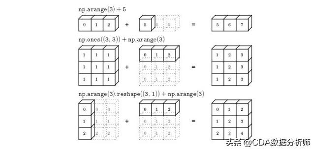
arr3是一个向量,能和标量1相加,是利用了"广播"机制.广播机制将标量1扩展为等长向量[1,1,1,1,1,1,1,1,1,1,]因此才实现了加法.

arr3 += 1
print(arr3)
# [ 1  2  3  4  5  6  7  8  9 10]

当我们想在指定区间内生成指定个数的数组时,如果利用np.arange()来生成,则需要手动计算步长.
其实可以用np.linspace()函数来解决.

• linspace(start, stop, num)
  左闭右闭,num指定均匀等分的数据个数. 注意arange是左闭右开.
  我们也可以指定endpoint = False来使区间变为左闭右开区间.

arr5 = np.linspace(0,10,20)
print(arr5)
'''
[ 0.          0.52631579  1.05263158  1.57894737  2.10526316  2.63157895
  3.15789474  3.68421053  4.21052632  4.73684211  5.26315789  5.78947368
  6.31578947  6.84210526  7.36842105  7.89473684  8.42105263  8.94736842
  9.47368421 10.        ]
'''

6.3.3 NumPy数组的其他常用函数

• zeros(), ones()生成的数组由0或1来填充. shape参数指定数组维度, dtype指定数据精度.
• full()生成任何形状

zeros = np.ones((3,4)) # (3,4)实际上是一个匿名的元组.
print(zeros)
'''
[[1. 1. 1. 1.]
 [1. 1. 1. 1.]
 [1. 1. 1. 1.]]
'''
 

ones = np.ones(shape = [4,3], dtype = int)
print(ones)
'''
[[1 1 1]
 [1 1 1]
 [1 1 1]
 [1 1 1]]
'''

• zeros_like(), ones_like()利用某个给定数组的类型尺寸,但所有元素都被替换为0或1
• empty_like()数组元素没有被初始化.
• full_like(a,value) 该数组a元素都被初始化为某个定值value,默认一维,shape参数指定类型

data2 = [(1,2,4,5,2),(21,2,7,3.2,1)]
data2_zeros = np.zeros_like(data2)
print(data2_zeros)
'''
[[0. 0. 0. 0. 0.]
 [0. 0. 0. 0. 0.]]
'''
data3 = [[1,3,23,4],[12,22,2,2],[1,3,5,7]]
arr6 = np.array(data3)
data3_ones = np.ones_like(arr6)
print(data3_ones)
'''
[[1 1 1 1]
 [1 1 1 1]
 [1 1 1 1]]
'''

np.full_like(arr5,9,shape = [4,5])
'''
array([[9., 9., 9., 9., 9.],
       [9., 9., 9., 9., 9.],
       [9., 9., 9., 9., 9.],
       [9., 9., 9., 9., 9.]])
'''

将数组重构的方法

• arr.reshape((2,3))
• arr.shape = (3,4)

print(data3_ones.reshape((2,6)))
data3_ones.shape = (1,12)
print(data3_ones)
# print(data3_ones.shape = (1,12))
'''
[[1 1 1 1 1 1]
 [1 1 1 1 1 1]]
[[1 1 1 1 1 1 1 1 1 1 1 1]]
'''

6.4 N维数组的属性

• ndim维度
• shape形状
• size大小(数组元素个数)

张量(Tensor)是矩阵在任意维度上的推广,张量的维度通常称为轴(axis)
多个矩阵可以构成一个新的3D向量,多个3D向量可以构成一个4D向量.
表达上,张量的方括号层次有多深,就表示这是多少维张量.

'''一维数组 又称1D张量 向量
形状用只含一个元素的元组表示

'''
my_array = np.arange(10)
print(my_array.ndim, my_array.shape, my_array.size)
# 1 (10,) 10
'''二维数组 又称2D张量 矩阵
形状第一个数字表示行,第二个数字表示列
'''
my_array = my_array.reshape((2,5))
print(my_array.ndim, my_array.shape, my_array.size)
# 2 (2, 5) 10

'''三维数组 又称3D张量
如果我们想创建两个三行五列的数组,它的形状参数为(2,3,5)
'''
a = np.arange(30).reshape((2,3,5))
print(a)
'''
[[[ 0  1  2  3  4]
  [ 5  6  7  8  9]
  [10 11 12 13 14]]

 [[15 16 17 18 19]
  [20 21 22 23 24]
  [25 26 27 28 29]]]
'''
print(a.ndim,a.shape,a.size)
# 3 (2, 3, 5) 30

6.5 NumPy数组中的运算

6.5.1 向量运算

6.5.2 算术运算

对相同形状的数组逐元素进行 + - * / % ** 运算
统计函数sum(), min(),average(),等 和 数学函数 sin(),cos()等

注:对于二维数组,维度信息必须一模一样.而矩阵乘法,不需要一模一样.我们可以将数组转换为矩阵来实现矩阵乘法.

arr_1 = np.arange(12).reshape((3,4))
arr_2 = np.linspace(1,12,12).reshape((3,4))
print(arr_1 / arr_2)
print(arr_1 * arr_2)
'''
[[0.         0.5        0.66666667 0.75      ]
 [0.8        0.83333333 0.85714286 0.875     ]
 [0.88888889 0.9        0.90909091 0.91666667]]
[[  0.   2.   6.  12.]
 [ 20.  30.  42.  56.]
 [ 72.  90. 110. 132.]]
'''

6.5.3 逐元素运算与张量点乘运算

数学上,不同形状的矩阵是可以进行乘法运算的,只要第一个矩阵的列和第二个矩阵的行相同就可以了. 矩阵乘法在NumPy里被称为dot()点乘

• dot(a, b)两个数组进行点乘运算 或者 a @ b 实现两个元素的矩阵乘法

import numpy as np
a = np.full_like(arr_1,2)
b = np.linspace(1,12,12).reshape((4,3))
c = np.dot(a,b)
print(f'{a}\n*\n{b}\n=\n{c}')
'''
[[2 2 2 2]
 [2 2 2 2]
 [2 2 2 2]]
*
[[ 1.  2.  3.]
 [ 4.  5.  6.]
 [ 7.  8.  9.]
 [10. 11. 12.]]
=
[[44. 52. 60.]
 [44. 52. 60.]
 [44. 52. 60.]]
'''

• mat()
  将数组转化成矩阵 然后直接相乘即可

a = np.mat(a)
b = np.mat(b)
a * b
'''
matrix([[44., 52., 60.],
        [44., 52., 60.],
        [44., 52., 60.]])
'''

rand = np.random.random((3,3))#创建0,1内随机数矩阵
'''
array([[0.74022509, 0.78820696, 0.26449078],
       [0.51691894, 0.03262771, 0.97027281],
       [0.47603836, 0.73180702, 0.20492381]])
'''

• 其他
  矩阵r.I 返回逆矩阵, r.T 返回转置矩阵, r.A, 返回矩阵对应的数组.
  np.eye()生成单位矩阵, np.diag()生成对角矩阵.

r = np.mat(rand)
print(f'逆矩阵:\n{r.I}\n转置矩阵\n{r.T}')
'''
逆矩阵:
[[ 4.87988147 -0.22224735 -5.24606218]
 [-2.46959989 -0.17887277  4.03438606]
 [-2.51674143  1.15505666  2.65920689]]
转置矩阵
[[0.74022509 0.51691894 0.47603836]
 [0.78820696 0.03262771 0.73180702]
 [0.26449078 0.97027281 0.20492381]]
'''

注意:如果矩阵的逆和矩阵相乘不是单位矩阵,很可能是矩阵不可逆.
如果np.linalg.det(矩阵)接近0则代表矩阵不可逆.

6.6 爱因斯坦求和约定

6.6.1 不一样的标记法

6.6.2 einsum()方法

用einsum()就能实现求和, 求外积, 求内积, 矩阵乘法, 矩阵转置, 求迹等操作.
如果我们用sum(), mat(), trace(), tensordot()来实现的话, 名称复杂, 进行高维度张量计算时容易出错.

输入格式字符->输出格式字符
格式字符串的字符数和张量的维数对应.ij代表二维张量,j表示一维张量,为空则表示0维张量即标量.

arr1 = np.arange(20).reshape((4,5))
print(arr1)
sum_col = np.einsum('ij->j',arr1)
print(sum_col)
sum_row = np.einsum('ab->a',arr1)
# sum_row = np.einsum('...a->...',arr1)
print(sum_row)
'''
[30 34 38 42 46]
[10 35 60 85]
'''

按照字符出现的顺序,i表示行j表示列,字符减少为1个,说明输出变量被降维了.而j被保留,它代表列,这说明行这个维度被消灭了.于是,这说明通过求和的方式达到维度约减.也就是上述操作实现了按列求和.
在格式字符串用什么字母不重要.ab->a完全没问题.
可以把没被约减掉的字母用…代替

einsum实现矩阵乘法

A = np.arange(1,10).reshape((3,3))
list1 = [1,3,5,3,2,4,1,0,1]
B = np.array(list1).reshape((3,3))
# print(A @ B)
'''
[[10  7 16]
 [25 22 46]
 [40 37 76]]
'''
result = np.einsum('ij,jk->ik',A,B)
print(result)
'''
[[10  7 16]
 [25 22 46]
 [40 37 76]]
'''

A,B对应格式字符串为ij,jk. 他们有相同的字符j,而j是A的列,B的行,说明j降维了,只有矩阵乘法才有类似的功效.

einsum()其他用法.

a = np.array([(1,2),(3,4)])
b = np.ones((2,2))
# a,b
print(a*b)# 对应元素相乘
print(np.einsum('ij,ij->ij',a,b))# 对应元素相乘
print(np.dot(a,b)) # 矩阵乘法
print(np.einsum('ij,ij->',a,b)) # 向量内积
print(np.einsum('ii->i',a))# 矩阵的迹
print(np.einsum('ij->ji',a))# 矩阵转置
'''
[[1. 2.]
 [3. 4.]]
[[1. 2.]
 [3. 4.]]
[[3. 3.]
 [7. 7.]]
10.0
[1 4]
[[1 3]
 [2 4]]
'''

6.7 NumPy中的轴方向

约减:并非减法之意,而是元素的减少.例如加法就是一种约减,因为他对众多元素按照加法指令实施操作,最后合并为少数的一个或几个值.例如sum,max,mean都是一种约减.
有的时候我们需要对某一维度的值进行统计,就需要给约减指定方向.

默认全维度约减, axis = 0竖直方向, axis = 1水平方向.
对于高维度数组而言,约减可以有先后顺序,因此axis的值还可以是一个向量,例如,axis = [0,1]表示先垂直后水平方向约减.

a = np.ones((2,3))
a.sum()# 6.0
a.sum(0)# array([2., 2., 2.]) 0代表垂直方向
a.sum(1) # array([3., 3.]) 1代表水平方向

对于高维数组, 应该是按括号层次来理解.括号由内到外,对应从小到大的维数.比如,对于一个三维的数组, 其维度由外到内分别为0,1,2.

[[[1,1,1],[2,2,2]],[[3,3,3],[4,4,4]]]

当我们指定sum()的axis = 0时,就是在第0个维度的元素之间进行求和操作,即拆掉最外层括号后对应的两个元素(在同一个层次)

[[1,1,1],[2,2,2]] 和 
[[3,3,3],[4,4,4]]

然后对同一个括号层次下的两个张量实施逐元素约减操作, 结果为

[[4,4,4],[6,6,6]]

若axis = 1 在第1个维度的元素之间进行求和操作
[1,1,1]和[2,2,2]在同一个括号(同一个维度)内相加,[3,3,3]和[4,4,4]在同一个括号内相加

剩下[[1,1,1],[2,2,2],[3,3,3],[4,4,4]]
[[3,3,3],[7,7,7]]

若axis = 2 在第2个维度的元素之间进行求和操作

[[1,1,1,2,2,2],[3,3,3,4,4,4]]

1,1,1在同一个维度,2,2,2在同一个维度…

[[3,6],[9,12]]

a = np.array([[[1,1,1],[2,2,2]],[[3,3,3],[4,4,4]]])
a.sum(axis = 0)
Out[28]:
array([[4, 4, 4],
       [6, 6, 6]])
In [29]:
a.sum(axis = 1)
Out[29]:
array([[3, 3, 3],
       [7, 7, 7]])
In [30]:
a.sum(axis = 2)
Out[30]:
array([[ 3,  6],
       [ 9, 12]])

b = [([(1,1),(2,2)],[(3,3),(4,4)]),([(5,5),(6,6)],[(7,7),(8,8)])]
b = np.array(b)
In [33]:
b.sum(0)
Out[33]:
array([[[ 6,  6],
        [ 8,  8]],
       [[10, 10],
        [12, 12]]])
In [34]:
b.sum(1)
Out[34]:
array([[[ 4,  4],
        [ 6,  6]],
       [[12, 12],
        [14, 14]]])
In [35]:
b.sum(2)
Out[35]:
array([[[ 3,  3],
        [ 7,  7]],
       [[11, 11],
        [15, 15]]])
In [36]:
b.sum(3)
Out[36]:
array([[[ 2,  4],
        [ 6,  8]],
       [[10, 12],
        [14, 16]]])

其他可实施约减的函数 如max,min和mean等,轴方向的约减也是类似的.

a = np.array([[[1,1,1],[2,2,2]],[[3,3,3],[4,4,4]]])
print(a.max(0),'\n\n',a.max(1),'\n\n',a.max(2),'\n\n',a.max())
'''
[[3 3 3]
 [4 4 4]] 

 [[2 2 2]
 [4 4 4]] 

 [[1 2]
 [3 4]] 

 4
'''

6.8 操作数组元素

6.8.1 通过索引访问数组元素

通过方括号访问,可反向访问.
访问二维数组的两种方法

• 像c/c++一样用两个方括号分别写出维度信息
• 在一个方括号内, 给出两个维度信息, 用逗号分割.

two_dim = np.linspace(1,9,9).reshape((3,3))

Out[3]:
array([[1., 2., 3.],
       [4., 5., 6.],
       [7., 8., 9.]])

In [5]:
two_dim[1][1] = 11
two_dim

Out[5]:
array([[ 1.,  2.,  3.],
       [ 4., 11.,  6.],
       [ 7.,  8.,  9.]])

In [6]:
two_dim[2,2] = 22
two_dim

Out[6]:
array([[ 1.,  2.,  3.],
       [ 4., 11.,  6.],
       [ 7.,  8., 22.]])

6.8.2 NumPy中的切片访问

• 和列表类似的操作
• 采取slice()函数实例化一个切片参数

a = np.arange(10)
s = slice(0,9,2)
b = a[s]
print(type(s),type(b))
print(a,s,b)
#<class 'slice'> <class 'numpy.ndarray'>
#[0 1 2 3 4 5 6 7 8 9] slice(0, 9, 2) [0 2 4 6 8]

6.8.3 二维数组的转置与展平

转置

• transpose()方法或T属性

展平

• ravel() 返回视图 原数组没有改变
• flatten() 深拷贝 原数组没有改变
• 显示变形 shape = (1,-1), -1表示列数是系统自动推导出来的,很常用.实际上还是二维数组,只是形状变了.

print(two_dim.ravel())
print(two_dim.flatten())
#[ 1.  2.  3.  4. 11.  6.  7.  8. 22.]
#[ 1.  2.  3.  4. 11.  6.  7.  8. 22.]
two_dim.shape = (1,-1)
print(two_dim)
#[[ 1.  2.  3.  4. 11.  6.  7.  8. 22.]]

6.9 NumPy中的广播

6.10 NumPy数组的高级索引

6.10.1 '‘花式’'索引

如果我们想访问多个元素, 而它们又没什么规律可循,就可以采用花式索引.

[0,0,0,4,5]为索引数组再作为数组a的下标, 达到访问多个元素的目的, 还可以访问重复的元素.

a = np.array([1,43,2,6,43,8,2,22,6,9])
fancy_array = a[[0,0,0,4,5]]
print(fancy_array)
#[ 1  1  1 43  8]
index = [0,0,0,4,5]
print(a[index]) # 可读性更强

花式索引访问二维数组的行

two_dim.shape = (3,3)
print(two_dim)
print(two_dim[[0,1,0]])
'''
[[ 1.  2.  3.]
 [ 4. 11.  6.]
 [ 7.  8. 22.]]
[[ 1.  2.  3.]
 [ 4. 11.  6.]
 [ 1.  2.  3.]]
'''

访问二维数组的列
需要用冒号添加一个维度.two_dim[:,col_index]表示所有行都涉及, 但列的访问范围由col_index来限定.这里冒号的用法来自数组切片.

col_index = [0,1,0]
print(two_dim[:,col_index])
'''
[[ 1.  2.  1.]
 [ 4. 11.  4.]
 [ 7.  8.  7.]]
'''

其他花式访问

print(two_dim[1,[0,1,0]])
# [ 4. 11.  4.]
row_index = [0,1,0]
col_index = [1,2,0]
print(two_dim[row_index,col_index])
# [2. 6. 1.]

掩码
有时候我们想要过滤一些不想要的元素.
列的掩码,是一个布尔类型,由于非零为真,因此np.array([1,0,1,0,1], dtype = bool)等价于
np.array([True,False,True,False,True])
下面使用了np.newaxis 相当于None.这里是为数组增加一个轴.

two_dim_arr = np.arange(20).reshape((4,5))
two_dim_arr
'''
array([[ 0,  1,  2,  3,  4],
       [ 5,  6,  7,  8,  9],
       [10, 11, 12, 13, 14],
       [15, 16, 17, 18, 19]])
'''
row_index = np.array([0,2,1]) #花式访问的行
col_mask = np.array([1,0,1,0,1], dtype = bool)#列的掩码
two_dim_arr[row_index[:,np.newaxis],col_mask]
'''
array([[ 0,  2,  4],
       [10, 12, 14],
       [ 5,  7,  9]])
'''

row_index[:,np.newaxis]将row_index从(3, )变成一个(3,1)伪二维数组,这样就相当于告诉numpy第一个参数无须和后面的参数拼接形成(行, 列)坐标对.
如果不这样写,row就是个一维的索引,numpy会把它和后面的参数进行拼接.形成二维数组的访问坐标.
再考虑到col_mask的站位和布尔属性,它实际上表示了哪些列可以取,哪些被过滤了.

row_index
Out[44]:array([0, 2, 1])
In [45]:row_index.shape
Out[45]:(3,)
In [46]:row_index[:,np.newaxis]
Out[46]:
		array([[0],
		       [2],
		       [1]])
In [47]:row_index[:,np.newaxis].shape
Out[47]:(3, 1)

two_dim_arr[row_index,col_mask]
# array([ 0, 12,  9])

a = np.arange(15).reshape(3,5)
a[a > 9]#array([10, 11, 12, 13, 14])

a是一个数组，9是标量，之所以能比较是因为广播技术。

a > 9
'''
array([[False, False, False, False, False],
       [False, False, False, False, False],
       [ True,  True,  True,  True,  True]])
'''

这个尺度与原始数组相同的数组，叫作布尔数组。布尔数组可以整体作为索引，形成一个布尔索引，然后numpy会根据逐元素规则, 返回对应位置布尔值为True的元素. 因此, a[a >9]的含义，就是返回数组中大于9的元素.

6.11 数组的堆叠操作

6.11.1 水平方向堆叠hstack()

hstack(tup),接收一个元组
concatenate(axis = 1), 可以完成同样的操作.

arr1 = np.zeros((2,2),dtype = int )
arr2 = np.ones((2,3),dtype = int )
np.hstack((arr1,arr2))
'''
array([[0, 0, 1, 1, 1],
       [0, 0, 1, 1, 1]])
'''

6.11.2 垂直方向堆叠vstack()

vstack(tup)垂直方向
concatenate(axis = 0)默认为0,即垂直方向

6.11.3 深度方向堆叠dstack()

在第三个维度堆叠

red = np.arange(9).reshape((3,3))
blue = np.arange(9,18).reshape((3,3))
green = np.arange(18,27).reshape((3,3))
print(red)
print(blue)
print(green)
print(np.dstack((red,blue,green)))
'''
[[0 1 2]
 [3 4 5]
 [6 7 8]]
[[ 9 10 11]
 [12 13 14]
 [15 16 17]]
[[18 19 20]
 [21 22 23]
 [24 25 26]]
[[[ 0  9 18]
  [ 1 10 19]
  [ 2 11 20]]

 [[ 3 12 21]
  [ 4 13 22]
  [ 5 14 23]]

 [[ 6 15 24]
  [ 7 16 25]
  [ 8 17 26]]]
'''

6.11.4 列堆叠与行堆叠

column_stack() 增加列 row_stack()增加行
列堆叠不等同于vstack垂直方向堆叠

一维数组堆叠

a = np.arange(3)
b = np.arange(3,6)
print(a)
print(b)
print(np.column_stack((a,b)))
print(np.vstack((a,b)))
print(np.row_stack((a,b)))
print(np.hstack((a,b)))
'''
[0 1 2]
[3 4 5]
[[0 3]
 [1 4]
 [2 5]]
[[0 1 2]
 [3 4 5]]
[[0 1 2]
 [3 4 5]]
[0 1 2 3 4 5]
'''

二维数组堆叠
column_stack == hstack
row_stack == vstack

print(np.column_stack((red,blue)))
print(np.vstack((red,blue)))
print(np.row_stack((red,blue)))
print(np.hstack((red,blue)))
'''
[[ 0  1  2  9 10 11]
 [ 3  4  5 12 13 14]
 [ 6  7  8 15 16 17]]
[[ 0  1  2]
 [ 3  4  5]
 [ 6  7  8]
 [ 9 10 11]
 [12 13 14]
 [15 16 17]]
[[ 0  1  2]
 [ 3  4  5]
 [ 6  7  8]
 [ 9 10 11]
 [12 13 14]
 [15 16 17]]
[[ 0  1  2  9 10 11]
 [ 3  4  5 12 13 14]
 [ 6  7  8 15 16 17]]
'''

6.11.5 数组的分割操作

split, hsplit, vsplit, dsplit

hsplit(array, indices_or_sections)水平方向分割(列分割)等价于split(axis = 1)
第一个参数表示被分割的数组, 第二个参数可为一个数或一个列表.
数表示等分的份数, 列表(矩阵)表示位置.
hsplit返回列表, 每个元素都是一个数组.

c = np.arange(16).reshape((4,4))
list1 = np.hsplit(c,4)
# type(list1) list
list1[1]
'''
array([[ 1],
       [ 5],
       [ 9],
       [13]])
'''

vsplit垂直方向或行方向上的分割.等同于split(axis = 0)
dsplit深度方向分割 等同于split(axis = 2)

array3 = np.arange(16).reshape(2,2,4)
array3
Out[35]:
array([[[ 0,  1,  2,  3],
        [ 4,  5,  6,  7]],
       [[ 8,  9, 10, 11],
        [12, 13, 14, 15]]])
In [36]:
np.dsplit(array3,2) # 分成了两个三维数组
Out[36]:
[array([[[ 0,  1],
         [ 4,  5]],
        [[ 8,  9],
         [12, 13]]]),
 array([[[ 2,  3],
         [ 6,  7]],
        [[10, 11],
         [14, 15]]])]
 np.dsplit(array3,[1,])
 [array([[[ 0],
         [ 4]],
        [[ 8],
         [12]]]),
 array([[[ 1,  2,  3],
         [ 5,  6,  7]],
        [[ 9, 10, 11],
         [13, 14, 15]]])]

6.12 NumPy中的随机数模块

np.random.seed(213)

np.random.randint(1,10,(2,3)) # 随机整数

Out[39]:

array([[5, 1, 2],
       [3, 7, 4]])

In [40]:

np.random.rand(2,3) # 生成均匀分布的随机数

Out[40]:

array([[0.91588577, 0.48486025, 0.87004422],
       [0.46589434, 0.86203022, 0.81577491]])

In [41]:

np.random.randn(2,3) # 生成标准正态分布的随机数

Out[41]:

array([[-1.35993274,  0.16770878,  0.69561962],
       [-1.05569746, -1.6872611 ,  0.9953465 ]])
       
# Two-by-four array of samples from N(3, 6.25):
# 生成均值为3,方差为6.25的随机数
>>> 3 + 2.5 * np.random.randn(2, 4)
array([[-4.49401501,  4.00950034, -1.81814867,  7.29718677],   # random
       [ 0.39924804,  4.68456316,  4.99394529,  4.84057254]])  # random

6.14 思考与提高

• csv 文本格式, 数据用逗号分割.行尾有\n
• join() 将序列中的元素以指定字符串连接生成一个新的字符串
  str.join(sequence)
• 生成文件需要加上encoding = 'utf-8’否则会出错

symbol = "-"
seq = ("a", "b", "c") # 字符串序列 
print(symbol.join( seq ))
# ','.join(seq)+'\n'
# 'a,b,c\n'

• 重塑为二维数组

two_dim_arr = np.arange(20).reshape((4,5))
two_dim_arr[:,0]
# array([ 0,  5, 10, 15])
two_dim_arr[:,[0]]
'''
array([[ 0],
       [ 5],
       [10],
       [15]])
'''

data_np[:,0].reshape(-1,1)# 重塑成了二维数组
'''
array([['2019/3/1 00:00'],
       ['2019/3/1 00:15'],
       ['2019/3/1 00:30'],
       ...,
       ['2019/5/31 22:30'],
       ['2019/5/31 22:45'],
       ['2019/5/31 23:00']], dtype='<U16')
'''

• np.column_stack(tup)

'''
会先把一维数组按列堆叠为二维数组
'''
'''
Stack 1-D arrays as columns into a 2-D array.

Take a sequence of 1-D arrays and stack them as columns
to make a single 2-D array. 2-D arrays are stacked as-is,
just like with `hstack`.  1-D arrays are turned into 2-D columns
first.
'''

按照NY, Ausin, Boulder三个城市, 将数据划分为三个文件,并以csv形式存储.

import numpy as np
data = []
with open('Grid, solar, and EV data from three homes.csv','r',encoding='utf-8') as file:
    lines = file.readlines()
    for line in lines:
        temp = line.split(',')
        data.append(temp)
# 分割表头
header = data[0]# 花式访问默认访问行
#分割数据
data_np = np.array(data[1:])
# 提取日期列(二维数组花式访问列)
date = data_np[:,0]
# 构建表头
NY_header = header[:4]
Austin_header = header[0:1] + header[4:7]
# header[0]取出的是字符串而非列表
# 注意字符串和列表无法相加 
# 用header[0:1]的方式取出仅包含一个元素的列表,然后相加
Boulder_header = [header[0]] + header[7:]
# 分割NY数据
NY_data = data_np[:,:4] # 二维数组,行全取,列取前四
with open('1-NY.csv','w',encoding='utf-8') as file:
    file.write(','.join(NY_header) + '\n') # 先把表头连起来
    for line in NY_data:
        file.write(','.join(line) + '\n')
Austin_data = np.hstack((data_np[:,0].reshape(-1,1), data_np[:, 4:7]))
# array不能像列表一样直接用+号相连,可以采用水平堆叠.
# np.hstack((data_np[:,0], data_np[:, 4:7]))
# all the input arrays must have same number of dimensions, but the array at index 0 has 1 dimension(s) and the array at index 1 has 2 dimension(s)

# np.hstack((data_np[:,[0]],data_np[:, 4:7])) # 这样也可以
with open('1-Austin.csv','w',encoding='utf-8') as file:
    file.write(','.join(Austin_header) + '\n')
    for line in Austin_data:
        file.write(','.join(line) + '\n')
Boulder_data = np.column_stack((data_np[:,0],data_np[:,7:]))
# column_stack会先把一维数组按列堆叠为二维数组,这样就不用转换了
with open('1-Boulder.csv','w',encoding='utf-8') as file:
    file.write(','.join(Boulder_header))
    for line in Boulder_data:
        file.write(','.join(line))

问题三个文件的数据都输出了12遍,(重新执行了一遍,好了)
第三个还有空行.(写文件的时候不加回车就好了)

• reader = csv.reader(f) 读文件对象
• writer = csv.writer(f) 写文件对象
• writer.writerows(out)写成csv文件自动加逗号回车

import csv
import numpy as np
from datetime import datetime
def power_stats(file):
    # 读取文件数据
    with open(file,'r') as f:
        reader = csv.reader(f)
        # 跳过空行
        data = [line for line in reader if len(line) > 0]
        
    #除掉表头,提取数据
    np_array = np.array(data[1:])
    #分割日期
    dates_str = np_array[:, 0]
    #分割用电数据
    elec_data = np_array[:, 1:]
    
    #数据预处理, 否则类型转换会出错
    elec_data[elec_data == ''] = '0'
    #转换数据类型
    elec_data = elec_data.astype(float)
    

    #转换为日期对象
    dates = [datetime.strptime(date,'%Y/%m/%d %H:%M') for date in dates_str]
#     print(dates) dates是datetime类型的列表
    #提取三个月份的数据索引
    index_m3 = [date.month == 3 for date in dates] # 布尔数组
    index_m4 = [date.month == 4 for date in dates]
    index_m5 = [date.month == 5 for date in dates]
#     print(index_m3)
    elec3 = elec_data[index_m3] # 每个月的电费列表
    elec4 = elec_data[index_m4]
    elec5 = elec_data[index_m5]
#     print(elec3)
#     m3_ratio = np.sum(elec3,axis = 0) / np.sum(elec3) # 列表 默认全维度约减, axis = 0竖直方向,
    m3_ratio = np.einsum('ij->j',elec3) / np.einsum('ij->',elec3)
    m4_ratio = np.sum(elec4,axis = 0) / np.sum(elec4)
    m5_ratio = np.sum(elec5,axis = 0) / np.sum(elec5)
#     print(np.sum(elec3),np.sum(elec3,axis = 0),m3_ratio)
    '''
    
    总量     每个部分的用电数据            占比
    4305.369 [1189.59  1073.14  2042.639] [0.27630384 0.24925622 0.47443994]
3192.221 [ 905.145  644.881 1642.195] [0.2835471 0.2020164 0.5144365]
2261.5 [1558.867  622.252   80.381] [0.68930665 0.27515012 0.03554322]
    '''
    return m3_ratio,m4_ratio,m5_ratio


filename = ['1-NY.csv','1-Austin.csv','1-Boulder.csv']
out = []
# [out.extend(power_stats(file)) for file in filename] b写法可读性太差
for file in filename:
    out.extend(power_stats(file))
# out
'''
[array([0.27630384, 0.24925622, 0.47443994]),
 array([0.18993516, 0.26238493, 0.54767991]),
 array([-0.14939335,  0.19007388,  0.95931948]),
 array([0.2835471, 0.2020164, 0.5144365]),
 array([0.27165157, 0.21153016, 0.51681827]),
 array([0.45301318, 0.15492749, 0.39205933]),
 array([0.68930665, 0.27515012, 0.03554322]),
 array([0.29504936, 0.19449082, 0.51045982]),
 array([0.32425077, 0.24613855, 0.42961069])]
'''
with open('./3.csv','w',encoding = 'utf-8') as f:
    writer = csv.writer(f)
    writer.writerows(out)

问题 生成的文件会有空行.
解决方法

1. : dialect = ‘unix’
2. : newline = ‘’

在Windows中：

‘\r’ 回车，回到当前行的行首，而不会换到下一行，如果接着输出的话，本行以前的内容会被逐一覆盖；

‘\n’ 换行，换到当前位置的下一行，而不会回到行首；

Unix系统里，每行结尾只有“<换行>”，即"\n"；Windows系统里面，每行结尾是“<回车><换行>”，即“\r\n”；Mac系统里，每行结尾是“<回车>”，即"\r"；。一个直接后果是，Unix/Mac系统下的文件在Windows里打开的话，所有文字会变成一行；而Windows里的文件在Unix/Mac下打开的话，在每行的结尾可能会多出一个^M符号。
解决方法1

在输出时，如果换行是None，则写入的任何’\ n’字符都被转换为系统默认行分隔符，os.linesep。 如果换行符是’‘(空字符)或’\ n’，不进行转换。 如果换行符是任何其他合法值【注意：不能将其随心所意地设置为其他英文字母，大家可以自行实验】，所有’\ n’字符都将被转换为给定的字符串。

如果newline采用默认值None（即不进行指定任何指定），在Windows系统下，os.linesep即为’\r\n’，那么此时就会将’\n’转换为’\r\n’（即CRLF），所以会多一个’\r’（回车）出来，即’\r\r\n’。在csv中打开就会多一行。

其他

• np.argsort(a)
  注意：返回的是元素值从小到大排序后的索引值的数组

In :       	a = np.array([3,1,2,1,3,5])
Out: 		[3,1,2,1,3,5] # 排序后 1 1 2 3 3 5 
		#索引0,1,2,3,4,5 #排序后索引1 3 2 0 4 5
In : 		b = np.argsort(a)                        # 对a按升序排列        
Out: 		[1 3 2 0 4 5]      

In : 		b = np.argsort(-a)                       # 对a按降序排列        
Out: 		[5 0 4 2 1 3]               	

• dtype = ‘<U1’

'''
   `<`表示字节顺序，小端（最小有效字节存储在最小地址中）
   
   `U`表示Unicode，数据类型
   
   `1`表示元素位长，数据大小
'''

7 Pandas数据分析

Pandas基于NumPy但是有比ndarray更为高级的数据结构Series(类似一维数组)和DataFrame(类似二维数组).
Panel(类似三维数组)不常用已经被列为过时的数据结构.

7.3 Series类型数据

7.3.1 Series的创建

series基于ndarray,因此必须类型相同.
pd.Series(data,index = index) index如果不写,默认从0~n-1

a = pd.Series([1,0,2,55])
'''
0     1
1     0
2     2
3    55
dtype: int64
'''
b = pd.Series([1,4,5.3,2,1],index = range(1,6))
'''
1    1.0
2    4.0
3    5.3
4    2.0
5    1.0
dtype: float64
'''

通过Series的index和values属性,分别获取索引和数组元素值.

a.values
Out[9]:array([ 1,  0,  2, 55], dtype=int64)
In [10]:a.index
Out[10]:RangeIndex(start=0, stop=4, step=1)

修改索引

a.index = ['a','b','c','d']
'''
a     1
b     0
c     2
d    55
dtype: int64
'''

利用字典创建Series
区别:字典无序,series有序. series的index和value之间相互独立.Series的index可变,字典的key不可变.

dict1 = {'a':1,'b':2,'c':3}
c = pd.Series(dict1)
'''
a    1
b    2
c    3
dtype: int64
'''

describe()方法

c.describe()
'''
count    3.0个数
mean     2.0均值
std      1.0均方差
min      1.0最小值
25%      1.5前25%的数据的分位数
50%      2.0
75%      2.5
max      3.0最大值
dtype: float64
'''

7.3.2 Series中的数据访问

采用方括号访问
索引号访问
索引值访问
用列表一次访问多个

c['a'] = 99
c[2] = 77
c
'''
a    99
b     2
c    77
dtype: int64
'''  
c[['a','b']]
'''
a    99
b     2
dtype: int64
'''

两个Series用append()方法叠加(append过时了,即将被移除,改用concat)
ignore_index=True重新添加索引

s1 = pd.Series([1,2,3])
s2 = pd.Series([4,5,6])
# s1.append(s2) 
# FutureWarning: The series.append method is deprecated and will be removed from pandas in a future version. Use pandas.concat instead.
pd.concat([s1,s2])
'''
0    1
1    2
2    3
0    4
1    5
2    6
dtype: int64
'''
pd.concat([s1,s2],ignore_index=True)
'''
0    1
1    2
2    3
3    4
4    5
5    6
dtype: int64
'''

7.3.3 Series中的向量化操作和布尔索引

c > c.mean()
'''
a     True
b    False
c     True
dtype: bool
'''

Series对象也可以作为numpy参数,因为本质上,Series就是一系列数据,类似数组向量.

s = pd.Series(np.random.random(5),['a','b','c','d','e'])
a = np.square(s)

7.3.4 Series中的切片操作

基于数字的切片左闭右开,基于标签的切片左闭右闭.

s[1:3]
'''
b    0.508859
c    0.524076
dtype: float64
'''
s[:'c']
'''
a    0.585969
b    0.508859
c    0.524076
dtype: float64
'''

7.3.5 Series中的缺失值

在 Pandas 中, 对于缺失值, 默认会以 NaN 这个 pandas 专属的标志来表示. 但它并不是一个 数字, 或字符串 或 None, 因此, 是 不能和空字符串 “” 来比较的.
pandas 中, 只能用 pd.isnull(), … 等几个相关的方法来判断 ‘空值’ NaN

arr = np.array([1,'a',3,np.nan])
t = pd.Series(arr)
'''
0      1
1      a
2      3
3    nan
dtype: object
'''

t.isnull()
'''
0    False
1    False
2    False
3    False
dtype: bool
'''

object类型数据的数组 isnull都会被判断为false, 改成float64也会被判断为false.只能重新赋值t[3] = np.nan

7.3.6 Series中的删除与添加操作

不会删除原有数据

t.drop(0)
t.drop([0,1,3])
'''
2    3.0
dtype: float64
'''
t
'''
0    1.0
1    2.0
2    3.0
3    NaN
dtype: float64
'''

如果我们想删除原有的数据加入inplace = True即可(本地)

t.drop(3,inplace=True)
'''
0    1.0
1    2.0
2    3.0
dtype: float64
'''

7.3.7 Series中的name属性

name与index.name 分别为数值列和索引列的名称

t.name = 'salary'
t.index.name = 'num'
'''
num
0    1.0
1    2.0
2    3.0
Name: salary, dtype: float64
'''

7.4 DataFrame类型数据

如果我们把Series看作Excel表中的一列, 那么DataFrame就是Excel中的一张表.从数据结构的角度看,Series好比一个带标签的一维数组,而DataFrame就是一个带标签的二维数组,它可以由若干一维数组(Series)构成.

7.4.1 构建DataFrame

DataFrame不仅有行索引还有列索引.

• 构建DataFrame最常用的方法是构建一个字典,
  再将字典作为DataFrame的参数.
  字典的key是DataFrame的列名称,字典的value是一个列表.列表的长度就是行数.

df1 = pd.DataFrame({'alpha':['a','b','c']})
'''
	alpha
0	a
1	b
2	c
'''

每个key都作为一列

dict2 = {'name':['a','b','c'],'age':[12,54,22],'address':['saddsa','aswww','xccc']}
df2 = pd.DataFrame(dict2)
df2
'''
	name	age	address
0	a	12	saddsa
1	b	54	aswww
2	c	22	xccc
'''

• 利用二维数组构建DataFrame
  此时DataFrame的行和列都是自然数序列

data1 = np.arange(9).reshape((3,3))
df3 = pd.DataFrame(data1)
df3
'''
	0	1	2
0	0	1	2
1	3	4	5
2	6	7	8
'''

显示指定列名和index行名

df4 = pd.DataFrame(data1,columns=['one','two','three'], index = ['a','b','c'])
df4
'''
	one	two	three
a	0	1	2
b	3	4	5
c	6	7	8
'''

读取index和columns行名和列名

df4.index

Out[11]:Index(['a', 'b', 'c'], dtype='object')

In [12]:df4.columns

Out[12]:Index(['one', 'two', 'three'], dtype='object')

• 利用Series构建

row1 = pd.Series(np.arange(3),index = ['a','b','c'])
row2 = pd.Series(np.arange(3,6), index = ['j','q','k'])
row1.name = 'series1'
row2.name = 'series2'
df5 = pd.DataFrame([row1, row2])
df5
'''
	a	b	c	j	q	k
series1	0.0	1.0	2.0	NaN	NaN	NaN
series2	NaN	NaN	NaN	3.0	4.0	5.0
'''

series的index(行)变成了DataFrame的列索引.数据缺失的地方用NaN代替了.

我们可以对DataFrame进行转置

df5.T
'''
series1	series2
a	0.0	NaN
b	1.0	NaN
c	2.0	NaN
j	NaN	3.0
q	NaN	4.0
k	NaN	5.0
'''

7.4.2 访问DataFrame中的列与行

常见访问方法
[ ]默认访问列
loc[ ]默认行
loc[: , ]逗号后面访问列
常用参数
index = 0 指定行
columns = 0 指定列
axis = 0 轴方向 默认行
inplace = False 是否本地操作
axis = ‘columns’ 或 axis = 1 列
axis = ‘index’ 或 axis = 0 行
ignore_index = False 默认忽略行索引

7.4.2.1 访问列

''' df4
	one	two	three
a	0	1	2
b	3	4	5
c	6	7	8
'''
df4.columns
# Index(['one', 'two', 'three'], dtype='object')
df4.columns.values
# array(['one', 'two', 'three'], dtype=object)

df4.columns返回的是index对象, df4.columns.values返回的是array对象.我们就可以访问数组下标了.

df4.columns.values[0]
# 'one'

如果我们已经知道DataFrame的列名,就可以以它作为索引读取对应的列.

  
df4['two']
'''
a    1
b    4
c    7
Name: two, dtype: int32
'''

DataFrame可以将列名作为DataFrame对象的属性来访问数据.

df4.three
'''
a    2
b    5
c    8
Name: three, dtype: int32
'''

但要注意 如果列名的字符串包含空格,或者名称不符合规范,那么就不能通过访问对象属性的方式来访问某个特定的列.

如果想要访问多个列, 还是得将列名打包到列表里,

df4[['one','two']]
'''
	one	two
a	0	1
b	3	4
c	6	7
'''

7.4.2.2 访问行

切片技术依据数字索引

df4[0:1]
'''
	one	two	three
a	0	1	2
'''
# df4[0]会报错

7.4.2.3 loc[]和iloc[]

loc[ ] 值索引访问
使用类似[ ]切片访问, 但是左闭右闭
访问索引为’a’的行

df4.loc['a']
'''
one      0
two      1
three    2
Name: a, dtype: int32
'''

访问两行数据

df4.loc[['a','b']]
'''
	one	two	three
a	0	1	2
b	3	4	5
'''

切片访问两行

df4.loc['b':'c']
'''
	one	two	three
b	3	4	5
c	6	7	8
'''

访问行列

df4.loc['b':'c','one':'two']
'''
	one	two
b	3	4
c	6	7
'''

iloc[ ] 按照数字索引访问

df4.iloc[1:,:2]
'''
	one	two
b	3	4
c	6	7
'''

访问第1行

df4.iloc[1]
'''
one      3
two      4
three    5
Name: b, dtype: int32
'''

7.4.3 DataFrame中的删除操作

和Series类似的drop()方法
index = 0 指定行
columns = 0 指定列
axis = 0 轴方向 默认行
inplace = False 是否本地操作
axis = ‘columns’ 或 axis = 1 删除列
axis = ‘index’ 或 axis = 0 删除行
注意仅返回视图

df5 = pd.DataFrame(np.linspace(1,9,9).reshape((3,3)), columns = ['one','two','three'],dtype='int64')

c3 = df5['three']
r3 = df5[2:3]
# (pandas.core.series.Series, pandas.core.frame.DataFrame)

df5.drop('three',axis='columns')
'''
	one	two
0	1	2
1	4	5
2	7	8
'''
# df5.drop('three',axis = 1)

df5.drop(0,axis = 'index')
'''
	one	two
1	4	5
2	7	8
'''
df5.drop(index = [0,1],columns=['one','two'])
'''
	three
2	9
'''

全局内置函数del 本地删除

del df5['three']
'''
	one	two
0	1	2
1	4	5
2	7	8
'''

7.4.4 DataFrame中的轴方向

axis = 1表示水平方向 (跨越不同的列columns, 列操作)
axis = 0表示垂直方向 (跨越不同的行index, 行操作)
类似numpy中的hstack等同于 column_stack

dff = pd.DataFrame(np.random.randint(1,12,size = (3,4)), columns=list('ABCD'))
'''
	A	B	C	D
0	4	2	9	7
1	1	7	5	2
2	6	10	6	9
'''
dff.max(axis = 1)
'''
0     9
1     7
2    10
dtype: int32
'''
dff.max(axis = 'index')
'''
A     6
B    10
C     9
D     9
dtype: int32
'''

7.4.5 DataFrame中的添加操作

7.4.5.1添加行

为一个原来没有的行索引赋值,实际上就是添加新行.

df6 = pd.DataFrame(columns=['属性1','属性2','属性3'])
for index in range(5):
    df6.loc[index] = ['name' + str(index)] + list(np.random.randint(10,size = 2))
    # 添加行 必须将字符串转换为列表 加方括号或者list函数均可
'''
	属性1	属性2	属性3
0	name0	2	6
1	name1	0	1
2	name2	1	4
3	name3	3	1
4	name4	8	8
'''
df6.loc['new_row'] = ['www',12,44]
'''
	属性1	属性2	属性3
0	name0	2	6
1	name1	0	1
2	name2	1	4
3	name3	3	1
4	name4	8	8
new_row	www	12	44
'''

添加多行数据

pd.concat([df6,df5],ignore_index=True)
'''
	one	two	three
0	name0	2	6.0
1	name1	0	1.0
2	name2	1	4.0
3	name3	3	1.0
4	name4	8	8.0
5	www	12	44.0
6	1	2	NaN
7	4	5	NaN
8	7	8	NaN
'''

7.4.5.2添加列

df5['three2'] = 3
'''
	one	two	three2
0	1	2	3
1	4	5	3
2	7	8	3
'''
df5.loc[:, 'four'] = np.random.randint(10,size = 3)
'''
one	two	three2	four
0	1	2	3	2
1	4	5	3	5
2	7	8	3	8
'''
pd.concat([df6,df5], axis = 'columns')
'''
	one	two	three	one	two	three2	four
0	name0	2	6	1.0	2.0	3.0	2.0
1	name1	0	1	4.0	5.0	3.0	5.0
2	name2	1	4	7.0	8.0	3.0	8.0
3	name3	3	1	NaN	NaN	NaN	NaN
4	name4	8	8	NaN	NaN	NaN	NaN
new_row	www	12	44	NaN	NaN	NaN	NaN
'''
# 也可以采用ignore_index = True 忽略列索引,重新赋值

7.5 基于Pandas的文件读取与分析

Pandas支持多种文件的读写

文件类型	读取函数	写入函数
csv	read_csv	to_csv
sql	read_sql	to_sql

7.5.1 利用Pandas读取文件

df = pd.read_csv('D:\study\code\Python\srcs\chap07-pandas\Salaries.csv')
'''
rank	discipline	phd	service	sex	salary
0	Prof	B	56	49	Male	186960
1	Prof	A	12	6	Male	93000
2	Prof	A	23	20	Male	110515
3	Prof	A	40	31	Male	131205
4	Prof	B	20	18	Male	104800
...	...	...	...	...	...	...
73	Prof	B	18	10	Female	105450
74	AssocProf	B	19	6	Female	104542
75	Prof	B	17	17	Female	124312
76	Prof	A	28	14	Female	109954
77	Prof	A	23	15	Female	109646
'''

read_csv方法的其他参数
sep = ‘,’ 默认逗号分割
index_col 指定某个列(比如ID,日期)作为行索引. 如果这个参数被设置为包含多个列的列表, 则表示设定多个行索引. 如果不设置则默认自然数0~n-1索引
delimiter 定界符(如果指定该参数,前面的sep失效)支持使用正则表达式来匹配某些不标准的csv文件.delimiter可视为sep的别名
converters 用一个字典数据类型指名将某些列转换为指定数据类型.在字典中,key用于指定特定的列, value用于指定特定的数据类型.
parse_dates 指定是否对某些列的字符串启用日期解析.如果字符串被原样加载,该列的数据类型就是object. 如果设置为True, 则这一列的字符串会被解析为日期类型.
header:指定行数作为列名 header = None 就是用自然数序列作为列名。这样就可以不把第一行数作为列名了。

7.5.2 DataFrame中的常用属性

• df.dtypes
  注:一列是Series要用dtype属性

df.dtypes
'''
rank          object
discipline    object
phd            int64
service        int64
sex           object
salary         int64
dtype: object
'''
df[['salary', 'sex']].dtypes
'''
salary     int64
sex       object
dtype: object
'''

在pandas ,object本质是字符串

In [12]:

df.columns # 查看DataFrame对象中各个列的名称

Out[12]:

Index(['rank', 'discipline', 'phd', 'service', 'sex', 'salary'], dtype='object')

In [13]:

df.axes # 返回行标签和列标签

Out[13]:

[RangeIndex(start=0, stop=78, step=1),
 Index(['rank', 'discipline', 'phd', 'service', 'sex', 'salary'], dtype='object')]

In [14]:

df.ndim # 返回维度数

Out[14]:

2

In [15]:

df.shape # 返回维度信息

Out[15]:

(78, 6)

In [16]:

df.size # 返回DataFrame元素个数

Out[16]:

468

In [17]:

df.values # 返回数值部分, 类似于一个没有行标签和列标签的numpy数组

Out[17]:

array([['Prof', 'B', 56, 49, 'Male', 186960],
       ['Prof', 'A', 12, 6, 'Male', 93000],
       ['Prof', 'A', 23, 20, 'Male', 110515],
       ['Prof', 'A', 40, 31, 'Male', 131205],
       ['Prof', 'B', 20, 18, 'Male', 104800],
       ['Prof', 'A', 20, 20, 'Male', 122400],
       ['AssocProf', 'A', 20, 17, 'Male', 81285],
       ['Prof', 'A', 18, 18, 'Male', 126300],
       ['Prof', 'A', 29, 19, 'Male', 94350],
       ['Prof', 'A', 51, 51, 'Male', 57800],
       ['Prof', 'B', 39, 33, 'Male', 128250],
       ['Prof', 'B', 23, 23, 'Male', 134778],
       ['AsstProf', 'B', 1, 0, 'Male', 88000],
       ['Prof', 'B', 35, 33, 'Male', 162200],
       ['Prof', 'B', 25, 19, 'Male', 153750],
       ['Prof', 'B', 17, 3, 'Male', 150480],
       ['AsstProf', 'B', 8, 3, 'Male', 75044],
       ['AsstProf', 'B', 4, 0, 'Male', 92000],
       ['Prof', 'A', 19, 7, 'Male', 107300],
       ['Prof', 'A', 29, 27, 'Male', 150500],
       ['AsstProf', 'B', 4, 4, 'Male', 92000],
       ['Prof', 'A', 33, 30, 'Male', 103106],
       ['AsstProf', 'A', 4, 2, 'Male', 73000],
       ['AsstProf', 'A', 2, 0, 'Male', 85000],
       ['Prof', 'A', 30, 23, 'Male', 91100],
       ['Prof', 'B', 35, 31, 'Male', 99418],
       ['Prof', 'A', 38, 19, 'Male', 148750],
       ['Prof', 'A', 45, 43, 'Male', 155865],
       ['AsstProf', 'B', 7, 2, 'Male', 91300],
       ['Prof', 'B', 21, 20, 'Male', 123683],
       ['AssocProf', 'B', 9, 7, 'Male', 107008],
       ['Prof', 'B', 22, 21, 'Male', 155750],
       ['Prof', 'A', 27, 19, 'Male', 103275],
       ['Prof', 'B', 18, 18, 'Male', 120000],
       ['AssocProf', 'B', 12, 8, 'Male', 119800],
       ['Prof', 'B', 28, 23, 'Male', 126933],
       ['Prof', 'B', 45, 45, 'Male', 146856],
       ['Prof', 'A', 20, 8, 'Male', 102000],
       ['AsstProf', 'B', 4, 3, 'Male', 91000],
       ['Prof', 'B', 18, 18, 'Female', 129000],
       ['Prof', 'A', 39, 36, 'Female', 137000],
       ['AssocProf', 'A', 13, 8, 'Female', 74830],
       ['AsstProf', 'B', 4, 2, 'Female', 80225],
       ['AsstProf', 'B', 5, 0, 'Female', 77000],
       ['Prof', 'B', 23, 19, 'Female', 151768],
       ['Prof', 'B', 25, 25, 'Female', 140096],
       ['AsstProf', 'B', 11, 3, 'Female', 74692],
       ['AssocProf', 'B', 11, 11, 'Female', 103613],
       ['Prof', 'B', 17, 17, 'Female', 111512],
       ['Prof', 'B', 17, 18, 'Female', 122960],
       ['AsstProf', 'B', 10, 5, 'Female', 97032],
       ['Prof', 'B', 20, 14, 'Female', 127512],
       ['Prof', 'A', 12, 0, 'Female', 105000],
       ['AsstProf', 'A', 5, 3, 'Female', 73500],
       ['AssocProf', 'A', 25, 22, 'Female', 62884],
       ['AsstProf', 'A', 2, 0, 'Female', 72500],
       ['AssocProf', 'A', 10, 8, 'Female', 77500],
       ['AsstProf', 'A', 3, 1, 'Female', 72500],
       ['Prof', 'B', 36, 26, 'Female', 144651],
       ['AssocProf', 'B', 12, 10, 'Female', 103994],
       ['AsstProf', 'B', 3, 3, 'Female', 92000],
       ['AssocProf', 'B', 13, 10, 'Female', 103750],
       ['AssocProf', 'B', 14, 7, 'Female', 109650],
       ['Prof', 'A', 29, 27, 'Female', 91000],
       ['AssocProf', 'A', 26, 24, 'Female', 73300],
       ['Prof', 'A', 36, 19, 'Female', 117555],
       ['AsstProf', 'A', 7, 6, 'Female', 63100],
       ['Prof', 'A', 17, 11, 'Female', 90450],
       ['AsstProf', 'A', 4, 2, 'Female', 77500],
       ['Prof', 'A', 28, 7, 'Female', 116450],
       ['AsstProf', 'A', 8, 3, 'Female', 78500],
       ['AssocProf', 'B', 12, 9, 'Female', 71065],
       ['Prof', 'B', 24, 15, 'Female', 161101],
       ['Prof', 'B', 18, 10, 'Female', 105450],
       ['AssocProf', 'B', 19, 6, 'Female', 104542],
       ['Prof', 'B', 17, 17, 'Female', 124312],
       ['Prof', 'A', 28, 14, 'Female', 109954],
       ['Prof', 'A', 23, 15, 'Female', 109646]], dtype=object)

7.5.3 DataFrame中的常用方法

head([n])返回前n行记录 默认为5
tail([n])返回后n行记录
describe(), max(), min(), mean(), median(), std()标准差
sample([n])随机抽n个样本, dropna() 将数据集合中所有含有缺失值的记录删除
value_counts() 查看某列中有多少个不同类别, 并可计算出每个不同类别在该列中有多少次重复出现, 实际上就是分类计数. ascending = True表示按升序排序. normalize = True可以看占比而非计数.
groupby()按给定条件进行分组

df.sex.value_counts()
'''
Male      39
Female    39
Name: sex, dtype: int64
'''
df.discipline.value_counts(ascending=True, normalize = True)
'''
A    0.461538
B    0.538462
Name: discipline, dtype: float64
'''

7.5.4 DataFrame的条件过滤

利用布尔索引获取DataFrame的子集.

# df[df.salary >= 130000][df.sex == 'Female']
# UserWarning: Boolean Series key will be reindexed to match DataFrame index.
df[(df.salary >= 130000) & (df.sex == 'Female')]
'''
	rank	discipline	phd	service	sex	salary
40	Prof	A	39	36	Female	137000
44	Prof	B	23	19	Female	151768
45	Prof	B	25	25	Female	140096
58	Prof	B	36	26	Female	144651
72	Prof	B	24	15	Female	161101
'''
df[(df.salary >= 130000) & (df.sex == 'Female')].salary.mean()
# 在DataFrame必须用& 不能用and
# and可能会报错
# 146923.2
df[(df['salary'] <= 100000) & (df['discipline'] == 'A')]['salary'].median()
# 77500.0

7.5.5 DataFrame的切片操作

DataFrame的切片操作和numpy的切片操作类型
之前的访问行和列就是一种切片.

df[5:15]
'''
rank	discipline	phd	service	sex	salary
5	Prof	A	20	20	Male	122400
6	AssocProf	A	20	17	Male	81285
7	Prof	A	18	18	Male	126300
8	Prof	A	29	19	Male	94350
9	Prof	A	51	51	Male	57800
10	Prof	B	39	33	Male	128250
11	Prof	B	23	23	Male	134778
12	AsstProf	B	1	0	Male	88000
13	Prof	B	35	33	Male	162200
14	Prof	B	25	19	Male	153750
'''

# df[5:15]['discipline':'sex']
# 报错cannot do slice indexing on RangeIndex with these indexers [discipline] of type str
df.loc[5:15,'discipline':'sex']# loc读取特定行和列的交叉左闭右闭
# loc可以这样写
'''
	discipline	phd	service	sex
5	A	20	20	Male
6	A	20	17	Male
7	A	18	18	Male
8	A	29	19	Male
9	A	51	51	Male
10	B	39	33	Male
11	B	23	23	Male
12	B	1	0	Male
13	B	35	33	Male
14	B	25	19	Male
15	B	17	3	Male
'''
df[5:15][['discipline','phd','service','sex']] # 切片左闭右开
'''
	discipline	phd	service	sex
5	A	20	20	Male
6	A	20	17	Male
7	A	18	18	Male
8	A	29	19	Male
9	A	51	51	Male
10	B	39	33	Male
11	B	23	23	Male
12	B	1	0	Male
13	B	35	33	Male
14	B	25	19	Male
'''

7.5.6 DataFrame的排序操作

• df.sort_values()
  by 指定按什么排序
  ascending = True 默认升序

df_sorted = df.sort_values(by = 'salary')
'''
rank	discipline	phd	service	sex	salary
9	Prof	A	51	51	Male	57800
54	AssocProf	A	25	22	Female	62884
66	AsstProf	A	7	6	Female	63100
71	AssocProf	B	12	9	Female	71065
57	AsstProf	A	3	1	Female	72500
'''

按service升序 salary降序

df_sorted = df.sort_values(by = ['service','salary'], ascending = [True,False])
df_sorted.head(10)
'''
rank	discipline	phd	service	sex	salary
52	Prof	A	12	0	Female	105000
17	AsstProf	B	4	0	Male	92000
12	AsstProf	B	1	0	Male	88000
23	AsstProf	A	2	0	Male	85000
43	AsstProf	B	5	0	Female	77000
55	AsstProf	A	2	0	Female	72500
57	AsstProf	A	3	1	Female	72500
28	AsstProf	B	7	2	Male	91300
42	AsstProf	B	4	2	Female	80225
68	AsstProf	A	4	2	Female	77500
'''

7.5.7 Pandas的聚合和分组运算

7.5.7.1 聚合

在pandas中聚合更侧重于描述将多个数据按照某种规则(即特定函数)聚合在一起, 变成一个标量的数据转换过程. 它与张量的约减(规约, reduce)有相通之处.

• agg()方法实现聚合操作,如果函数名是官方提供的则以字符串的形式给出,如果来自第三方(如numpy)或自己定义的,则直接给出函数的名称(不得用引号括起来).

df['salary'].agg(['max', np.min, 'mean', np.median])
'''
max       186960.000000
amin       57800.000000
mean      108023.782051
median    104671.000000
Name: salary, dtype: float64
'''
df[['salary']].agg(['max', np.min, 'mean', np.median])
'''
salary
max	186960.000000
amin	57800.000000
mean	108023.782051
median	104671.000000
'''

其他统计函数

• mode()众数
• skew() 偏度
• kurt() 峰度

偏度和峰度用于检测数据集是否满足正态分布
偏度的衡量是相对于正态分布来说的, 正态分布的偏度为0.若带分析的数据分布是对称的, 那么偏度接近于0, 若偏度大于0, 则说明数据分布右偏, 即分布有一条长尾在右. 若偏度小于0, 则数据分布左偏.
峰度是体现数据分布陡峭或平坦的统计量.正态分布的峰度为0.若峰度大于0.表示该数据分布与正态分布相比较为陡峭, 有尖顶峰. 若峰度小于0, 表示该数据分布与正态分布相比较为平坦, 曲线有平顶峰.

df[['service','salary']].agg(['skew','kurt'])
'''
		service	    salary
skew	0.913750	0.452103
kurt	0.608981	-0.401713
'''

agg可以针对不同的列给出不同的统计, 这时, agg()方法内的参数是一个字典对象.

df.agg({'salary':['max','min'], 'service':['mean','std']})
'''
	salary	service
max	186960.0	NaN
min	57800.0	    NaN
mean	NaN	15.051282
std	    NaN	12.139768
'''

7.5.7.2 分组

• groupby()
  生成DataFrameGroupBy对象, 要想让其发挥作用, 还需要将特定方法应用在这个对象上, 这些方法包括但不限于 mean(), count(), median()等

df.groupby('rank').sum()
'''
	phd	service	salary
rank			
AssocProf	196	147	1193221
AsstProf	96	42	1545893
Prof	1245	985	5686741
'''
df.groupby('rank').describe() # 返回按rank分组的描述

df.groupby('rank')['salary'].mean() # 单层方括号是Series
'''
rank
AssocProf     91786.230769
AsstProf      81362.789474
Prof         123624.804348
Name: salary, dtype: float64
'''
df.groupby('rank')[['salary']].mean() # 双层方括号括起来是DataFrame
'''
	salary
rank	
AssocProf	91786.230769
AsstProf	81362.789474
Prof	123624.804348
'''

df.groupby('rank')[['service', 'salary']].agg(['sum','mean','skew'])
'''
	service	salary
sum	mean	skew	sum	mean	skew
rank						
AssocProf	147	11.307692	1.462083	1193221	91786.230769	-0.151200
AsstProf	42	2.210526	0.335521	1545893	81362.789474	0.030504
Prof	985	21.413043	0.759933	5686741	123624.804348	0.070309
'''

犯的错误和测试

# type(df.groupby('rank'))
# pandas.core.groupby.generic.DataFrameGroupBy

# type(df.groupby('rank').agg('mean'))
# pandas.core.frame.DataFrame

# type(df.groupby('rank').agg(['mean','sum']))
# FutureWarning: ['discipline', 'sex'] did not aggregate successfully. If any error is raised this will raise in a future version of pandas. Drop these columns/ops to avoid this warning.

# type(df.groupby('rank')['sex'])
# pandas.core.groupby.generic.SeriesGroupBy

# type(df.groupby('rank')[['sex','salary']])
# pandas.core.groupby.generic.DataFrameGroupBy

# df.groupby('rank')[['service','salary']].agg(['mean','kurt'])
# 如果要用统计方法mean,max等,要确保选取的列都是数值型的
# 因为每一列都是一个series 而series没有kurt方法

df.groupby('rank')[['service','salary']].agg(['mean'])
'''
			service	salary
			mean	mean
rank		
AssocProf	11.307692	91786.230769
AsstProf	2.210526	81362.789474
	Prof	21.413043	123624.804348
'''
# 不一样 虽然我也说不出来为什么
df[['service','salary']].agg(['skew','kurt'])
'''
		service	    salary
skew	0.913750	0.452103
kurt	0.608981	-0.401713
'''
df[['service','salary']].kurt() # 这样可以
df.groupby('rank')[['service','salary']].kurt() # 这会报错
df.groupby('rank')[['service','salary']].mean() # 这样也可以

7.5.8 DataFrame的透视表

透视表(pivot table)是一种常见的数据汇总工具, 可以根据一个键或多个键对数据进行聚合, 并根据行和列上的分组键将数据分配到不同的矩形区域中. 之所以称为透视表, 是因为我们可以动态地改变数据的位置分布, 以便按照不同方式分析数据, 它也支持重新安排行号, 列标和字段.
pd.pivot_table() pandas的全局函数
data 数据源
values 用于聚合操作的列
index 行层次的分组依据 一个值或多个值
columns 列层次的分组依据
aggfunc 对数据执行聚合操作时所用的函数, 默认 aggfunc = ‘mean’
注: 对象df本身就有成员方法, df.pivot_table(index = ‘rank’)
把职称作为index而非自然数序列

pd.pivot_table(df,index='rank')
'''
				phd	salary	service
	rank			
AssocProf	15.076923	91786.230769	11.307692
AsstProf	5.052632	81362.789474	2.210526
	Prof	27.065217	123624.804348	21.413043
'''

看看不同职称男女教师的薪资差异, 设置二级index来完成数据透视.
index就是数据划分的层次字段(key)

df.pivot_table(index = ['rank','sex'])
'''
							phd	salary	service
	rank	sex			
AssocProf	Female	15.500000	88512.800000	11.500000
			Male	13.666667	102697.666667	10.666667
AsstProf	Female	5.636364	78049.909091	2.545455
			Male	4.250000	85918.000000	1.750000
	Prof	Female	23.722222	121967.611111	17.111111
			Male	29.214286	124690.142857	24.178571
'''

将行列实施转置

• df.unstack()将行转为列
• df.stack()将列转为行
  如果不指定索引级别,stack()和unstack()默认对最内层进行操作(即level = -1, 这里的 -1表示倒数第一层).
  stack()和unstack()为一组逆运算操作.
  将内层索引sex转置为列

df.pivot_table(index = ['rank','sex']).unstack()
'''
			phd	salary	service
sex	Female	Male	Female	Male	Female	Male
rank						
AssocProf	15.500000	13.666667	88512.800000	102697.666667	11.500000	10.666667
AsstProf	5.636364	4.250000	78049.909091	85918.000000	2.545455	1.750000
	Prof	23.722222	29.214286	121967.611111	124690.142857	17.111111	24.178571
'''

values用来指定特定字段,从而筛选列.

df.pivot_table(index = ['rank','sex'], values = 'salary')
'''
			salary
rank	sex	
AssocProf	Female	88512.800000
			Male	102697.666667
AsstProf	Female	78049.909091
			Male	85918.000000
	Prof	Female	121967.611111
			Male	124690.142857
'''

df.pivot_table(index = ['rank','sex'], values = ['salary', 'service'], aggfunc = [np.sum, 'mean'])
'''
			sum	            mean
			salary	service	salary	service
rank	sex				
AssocProf	Female	885128	115	88512.800000	11.500000
			Male	308093	32	102697.666667	10.666667
AsstProf	Female	858549	28	78049.909091	2.545455
			Male	687344	14	85918.000000	1.750000
	Prof	Female	2195417	308	121967.611111	17.111111
			Male	3491324	677	124690.142857	24.178571
'''

透视表和groupby在很多方面的功能都是等价的.

df.groupby(['rank','sex'])[['salary','service']].agg(['sum', 'mean'])
# 上面写法和此句几乎完全等价
'''略有不同
					salary	service
				sum	mean	sum	mean
rank	sex				
AssocProf	Female	885128	88512.800000	115	11.500000
			Male	308093	102697.666667	32	10.666667
AsstProf	Female	858549	78049.909091	28	2.545455
			Male	687344	85918.000000	14	1.750000
	Prof	Female	2195417	121967.611111	308	17.111111
			Male	3491324	124690.142857	677	24.178571
'''

7.5.9 DataFrame的类SQL操作

query(查询字符串)方法实现 对行操作, 注意要加引号, 而且查询的是字符串还要加不同的引号.包括单引号,双引号,三单引号,三双引号.

df[df['rank'] == 'Prof'].head(10)
# 等价于
df.query("rank == 'Prof'").head(10)
# df.query('''rank == "Prof"''').head(10)
df.query('phd == 5')
df.query('rank == "Prof" and discipline == "A" and sex == "Male" ')

使用外部定义的变量 @必不可少

dis = 'B'
df.query("discipline == @dis ").head()

7.5.10

缺失值检测isnull 和notnull
缺失值填充fillna(x) 默认填充0 na表示缺失值
缺失值丢弃dropna() 丢弃含空值的行列.
函数形式：dropna(axis=0, how=‘any’, thresh=None, subset=None, inplace=False)
参数：
axis：轴。0或’index’，表示按行删除；1或’columns’，表示按列删除。
how：筛选方式。‘any’，表示该行/列只要有一个以上的空值，就删除该行/列；‘all’，表示该行/列全部都为空值，就删除该行/列。
thresh：非空元素最低数量。int型，默认为None。如果该行/列中，非空元素数量小于这个值，就删除该行/列。
subset：子集。列表，元素为行或者列的索引。如果axis=0或者‘index’，subset中元素为列的索引；如果axis=1或者‘column’，subset中元素为行的索引。由subset限制的子区域，是判断是否删除该行/列的条件判断区域。
inplace：是否原地替换。布尔值，默认为False。如果为True，则在原DataFrame上进行操作，返回值为None。

a = np.ones((11,10))
for i in range(len(a)):
    a[i,:i] = np.nan
 
d = pd.DataFrame(data = a)
print(d)
'''
    0    1    2    3    4    5    6    7    8    9
0   1.0  1.0  1.0  1.0  1.0  1.0  1.0  1.0  1.0  1.0
1   NaN  1.0  1.0  1.0  1.0  1.0  1.0  1.0  1.0  1.0
2   NaN  NaN  1.0  1.0  1.0  1.0  1.0  1.0  1.0  1.0
3   NaN  NaN  NaN  1.0  1.0  1.0  1.0  1.0  1.0  1.0
4   NaN  NaN  NaN  NaN  1.0  1.0  1.0  1.0  1.0  1.0
5   NaN  NaN  NaN  NaN  NaN  1.0  1.0  1.0  1.0  1.0
6   NaN  NaN  NaN  NaN  NaN  NaN  1.0  1.0  1.0  1.0
7   NaN  NaN  NaN  NaN  NaN  NaN  NaN  1.0  1.0  1.0
8   NaN  NaN  NaN  NaN  NaN  NaN  NaN  NaN  1.0  1.0
9   NaN  NaN  NaN  NaN  NaN  NaN  NaN  NaN  NaN  1.0
10  NaN  NaN  NaN  NaN  NaN  NaN  NaN  NaN  NaN  NaN 
'''
print(d.dropna(axis = 'columns', thresh=5))
'''
	  4    5    6    7    8    9
0   1.0  1.0  1.0  1.0  1.0  1.0
1   1.0  1.0  1.0  1.0  1.0  1.0
2   1.0  1.0  1.0  1.0  1.0  1.0
3   1.0  1.0  1.0  1.0  1.0  1.0
4   1.0  1.0  1.0  1.0  1.0  1.0
5   NaN  1.0  1.0  1.0  1.0  1.0
6   NaN  NaN  1.0  1.0  1.0  1.0
7   NaN  NaN  NaN  1.0  1.0  1.0
8   NaN  NaN  NaN  NaN  1.0  1.0
9   NaN  NaN  NaN  NaN  NaN  1.0
10  NaN  NaN  NaN  NaN  NaN  NaN
'''

7.6 泰坦尼克幸存者数据预处理

7.6.2 数据集的拼接

训练集 train.csv 测试集 test.csv

train_df = pd.read_csv('./titanic/train.csv')
train_df.info()
train_df.describe()
train_df.isnull().sum()
test_df = pd.read_csv('./titanic/test.csv')
full_df = pd.concat([train_df, test_df], ignore_index=True, sort=False)

concat 参数join默认外连接(没有为NaN), 内连接是只取交集
axis = 0 默认垂直方向合并
测试集没有Survived(因为这是留给训练好的模型来预测的)这一列, 所以会被设置为NaN. 之后可以依据此进行分割.

7.6.3 缺失值的处理

fillna()
value填充值, 默认为None.
method 填充策略 ‘backfill’或’bfill’ 则表示在填充时会按照指定的轴方向, 向回找到上一个合法有效的值,然后填充之. 如果为’ffill’或’pad’ 则表示按照指定的轴方向,向前找到一个有效值来填充.
axis 轴方向 inplace 本地

full_df[‘Embarked’]返回一个Series对象, 我们这里mode()求众数,由于众数有可能有多个,因此采用mode()[0]获取列表第一个元素.
对于Age列采用平均值填充, 怎么填充取决于你对数据处理的偏好, 并无好坏之分.

full_df['Embarked'].isnull().sum() # 2
full_df['Embarked'].fillna(full_df['Embarked'].mode()[0], inplace = True)
full_df['Embarked'].isnull().sum() # 0
full_df['Age'].isnull().sum() # 263
full_df['Age'].fillna(full_df['Age'].mean(), inplace = True)
full_df['Age'].isnull().sum() # 0

full_df.isnull().sum()
'''
PassengerId       0
Survived        418
Pclass            0
Name              0
Sex               0
Age               0
SibSp             0
Parch             0
Ticket            0
Fare              1
Cabin          1014
Embarked          0
dtype: int64
'''
full_df.isnull().count() # 不要被误解了, count只是计数 不管是否为0
'''
PassengerId    1309
Survived       1309
Pclass         1309
Name           1309
Sex            1309
Age            1309
SibSp          1309
Parch          1309
Ticket         1309
Fare           1309
Cabin          1309
Embarked       1309
dtype: int64
'''

看看哪些字段还缺失

percent_1 = full_df.isnull().sum() / full_df.isnull().count() * 100# 缺失率
percent_2 = round(percent_1, 2).sort_values(ascending = False)# round python内置函数 也可以用pandas 的round方法
# 按降序排列
# percent_2就是将percent_1 四舍五入再排序了一下 代表为空的占总个数的比例
full_df.isnull().sum().sort_values(ascending = False)
total = full_df.isnull().sum().sort_values(ascending = False)
# 代表为空的个数
missing_data = pd.concat([total, percent_2], axis = 1,
                         keys = ['Total','%'])
missing_data.head()

full_df['Fare'].fillna(full_df['Fare'].mean(),inplace = True)

Cabin缺失较多, 我们可以抛弃, 但是这可能是一个有用的特征, 我们要将其保留, 处理为有或没有房间号两大类, 没有房间号的用’NA’ 填充 NA表示not available

full_df['Cabin'].isnull().sum() # 1014
# Cabin不能丢弃 保留 分为有房间和无房间
full_df['Cabin'].fillna('NA', inplace = True)
full_df['Cabin'].isnull().sum() # 0

将处理完后的数据分别存起来.

train_clean = full_df[full_df['Survived'].notnull()]# 利用布尔索引 仅保留Survived不为NaN的行
train_clean.to_csv('train_clean.csv')
test_clean = full_df[full_df['Survived'].isnull()]# 保留为NaN的行
test_clean.to_csv('test_clean.csv')

7.8 思考与提高

1将数据进行转置， 转置后形如eg.csv, 缺失值用NAN代替.

# 标准写法
df = pd.read_csv('data.csv', parse_dates = True, index_col = [0, 1])
df.head()
'''
					KWH
CONS_NO	DATA_DATE	
1	    2015-01-01	6.68
		2015-01-02	2.50
		2015-01-03	5.20
		2015-01-04	4.17
		2015-01-05	4.89
'''
# 将行索引转成列,默认最内(level = -1) 可不能转置,转置和题目要求就不一样了
# 这里.KWH是因为只有KWH属性,就没必要显示了,按题目的要求.
df = df.unstack().KWH
'''
DATA_DATE	2015-01-01	2015-01-02	2015-01-03	2015-01-04	2015-01-05	...
CONS_NO																	
1	6.68	2.50	5.20	4.17	4.89	5.26	4.11	3.70	...
2	1.22	0.65	1.14	1.04	1.33	1.02	0.08	0.09	...
3	7.35	6.65	7.76	4.02	4.68	7.06	6.51	7.00	...
4	0.62	1.92	0.65	1.30	0.71	1.36	0.89	1.24	...
5	2.58	2.60	2.36	1.83	2.05	1.97	1.98	1.44	...
'''
# 缺失值用nan填充
df.fillna(np.nan, inplace = True)

8 Matplotlib与Seaborn可视化分析

8.1 Matplotlib与图形绘制

matplotlib可以很轻松的分析条形图, 散点图, 饼图等专业图形. 但是不够细腻, 比较底层.
Seaborn绘图库 图形更加细腻,更加高大上.

8.2 绘制简单图形

Pyplot是Matplotlib的子库, 很方便的让用户绘制2D图.

np中的sin函数,向量进向量出 给进去一个向量x,sin(x)批量产生一个相同维度的向量y
plot用于绘制线图和散点图
画单条线
plot([x], y, [fmt], *, data=None, **kwargs)
画多条线
plot([x], y, [fmt], [x2], y2, [fmt2], …, **kwargs)

nbSamples = 64
x = np.linspace(-math.pi, math.pi, nbSamples)
y1 = np.sin(x)
y2 = np.cos(x)
plt.plot(x, y1)
plt.show()
plt.plot(x, y1, 'r+:')

A format string consists of a part for color, marker and line:
fmt = ‘[marker][line][color]’
颜色
线形 - 代表实线, --短划线 -.点画线 : 电线

color=['b','g','r','c','m','y','k','w']
linestyle=['-','--','-.',':']

点形

marker=['.',',','o','v','^','<','>','1','2','3','4','s','p','*','h','H','+','x','D','d','|','_','.',',']

其他

# 蓝色,线宽20,圆点,点尺寸50,点填充红色,点边缘宽度6,点边缘灰色
plt.plot(y,color="blue",linewidth=20,marker="o",markersize=50,
         markerfacecolor="red",markeredgewidth=6,markeredgecolor="grey")

8.3 pyplot的高级功能

8.3.1添加图例与注释

• plt.legend() 添加注释
  对不同的图添加图例legend, loc是位置的缩写, best表示最佳位置, 也可以设置upper right(右上) center(中)等等.
  label是轴的标题, title是图像的标题, legend是图像的图例 两个$包裹公式, 生成latex风格的公式
  字符串前的r表示raw,即后面的字符串不需要转义

plt.plot(x, y1, color = 'red', linestyle = '--', linewidth = 4, label = r'y = sin(x)')
plt.plot(x, y2, '*', markersize = 8, markerfacecolor = 'r', markeredgecolor = 'b', label = r'$y = cos(x)$')
plt.legend(loc = 'best')
plt.show()

显示坐标点
plt.text(a, b, (a, b), ha = ‘center’, va = ‘bottom’, fontsize = 10)
显示文本注释
前两个参数表示x轴和y轴的坐标位置, 第三个参数表示标注的文本内容, 我们在这里打算显示的是坐标点.
可以调整前两个参数的位置以优化文本的位置.
ha, va分别是水平对齐(horizontal alignment)和垂直对齐.
ha可选的参数有 center, right, left,
va可选的参数有 center, top, bottom, baseline, center_baseline

x = np.arange(0,10)
y = 2 * x
for a, b in zip(x, y):
    plt.text(a - 0.5, b, (a, b), ha = 'center', va = 'bottom', fontsize = 10)
    
plt.plot(x, y, 'bo-')
plt.show()

8.3.2设置图形标题及坐标轴

• rcParams rc配置或rc参数
  可以修改默认的属性，包括窗体大小、每英寸的点数、线条宽度、颜色、样式、坐标轴、坐标和网络属性、文本、字体等。rc参数存储在字典变量中，通过字典的方式进行访问。
• plt.title() 设置图形标题
• plt.xticks() 设置x轴刻度
• plt.xlim() 设置x轴的区间范围
• plt.xlabel() 设置x轴名称

x = np.arange(-5, 5, 0.05)
y1 = np.sin(x)
y2 = np.cos(x)
# 为在matplotlib中显示中文, 设置特殊字体
plt.rcParams['font.sans-serif'] = ['SimHei'] # 正常显示中文标签
plt.rcParams['axes.unicode_minus'] = False # 正常显示负号
plt.title('双曲线')

plt.ylim(-1.2, 1.2)# 比-1,1大一点就可以了
plt.xlim(-6, 6)
plt.xticks(ticks = np.arange(-1.5 * np.pi, 2*np.pi, 0.5*np.pi),
          labels = ['$-\\frac{3}{2}\pi$','$-\pi$','$-\\frac{1}{2}\pi$',
                   '0', '$\\frac{1}{2}\pi$', '$\pi$','$\\frac{3}{2}\pi$'])
# ticks设置坐标轴的刻度,labels设置坐标轴的标签
plt.yticks(ticks = [-1,0,1])#设置刻度
plt.xlabel('我是$x$轴')#设置轴标签名
plt.ylabel('我是$y$轴')

plt.plot(x, y1, 'r',label = '$y_1 = sin(x)$')
plt.plot(x, y2, 'b:', label = '$y_2 = cos(x)$')

plt.legend(loc = 'best')
# plt.show()
# plt.savefig('sincos.jpg',dpi = 600)
# 把图片保存起来,dpi是分辨率 不是必须的

8.3.3 添加网格线

grid() 参数visible表示网格是否可见, which = [‘major’|‘minor’|‘both’](大网格|小网格|大网格套小网格)
axis = ‘x’|‘y’|‘both’ 表示在哪个轴添加网格线

data = np.arange(0,4,0.2)
plt.plot(data, data, 'r-.', data, data**2, 'bs', data, data**3, 'g^')
# plt.show()
plt.grid(visible = True, axis = 'y')

8.3.4 绘制多个子图

• plt.subplot(nrow,ncols,plot_number)
• fig.add_subplot()画布添加子图

nrows行ncols列的第plot_number个子图
例如 subplot(2,1,1)表示两行一列的第一个子图可简写为 subplot(211) （从 1 开始）

def f(t):
    return np.exp(-t) * np.cos(2 * np.pi * t)

t1 = np.arange(0, 5, 0.1)
t2 = np.arange(0, 5, 0.02)
# 第一种绘制子图的方法
fig = plt.figure() # 创建一个画布
sub_fig1 = fig.add_subplot(211) # 在画布上创建一个子图
sub_fig1.grid(True)
plt.plot(t1, f(t1), 'bo', t2, f(t2), 'k')

#第二种绘制子图的方法
plt.subplot(2,1,2)
plt.plot(t2, np.cos(2*np.pi*t2), 'r--')

8.3.5 Axes与Subplot的区别

figure画布最大.在画布里,我们可以创建各种子图, 子图主要有两类,一类是规矩排列整齐的子图,叫做Subplot,另一类是可以不那么规则摆放的子图,叫做Axes
本质上,axes更加底层,事实上,subplot也是调用axes来实现的,不过是子图排列的更加规范罢了,因为subplot某种程度上是axes的特例.
可能matplotlib的设计者认为,任何一个子图都要通过多个轴来呈现,所以就用Axes来表示子图,但切不可认为axes是多个轴的意思.
axes.set_xlabel()

fig = plt.figure()
left1, bottom1, width1, height1 = 0.1, 0.1, 0.8, 0.8
# 在画布上添加一个子图 必须给出子图的位置用四个点的列表确定
#左下角的位置即图原点的x,y坐标和图的宽度和高度
axes_1 = fig.add_axes([left1, bottom1, width1, height1])
axes_1.scatter(x, y)
axes_1.set_xlabel('x')
axes_1.set_ylabel('y')
axes_1.set_title('title')

left2, bottom2, width2, height2 = 0.6, 0.6, 0.25, 0.25
# 添加另一个子图
axes_2 = fig.add_axes([left2, bottom2, width2, height2])
axes_2.plot(x,y)
axes_2.set_title('title_inside')
plt.show()

• fig.add_axes([left1, bottom1, width1, height1])
  左下角的位置即图原点的x,y坐标和图的宽度和高度
  这四个值都用占整个figure坐标系的百分比来表示, 即都是小于1的小数.
  用add_axes()方法生成子图更加灵活,完全可以实现add_subplot()方法的功能, 且更容易控制子图的显示位置, 甚至实现相互重叠的效果.

x = np.linspace(0, 2*np.pi, 400)
y = np.sin(x**2)
fig = plt.figure()
left, bottom, width, height = 0.1, 0.1, 0.5, 0.5
axes_1 = fig.add_axes([left, bottom, width, height])
axes_2 = fig.add_axes([left + 0.1, bottom + 0.1, width, height])
axes_3 = fig.add_axes([left+0.2, bottom+0.2, width, height])
axes_4 = fig.add_axes([left+0.3, bottom+0.3, width, height])
axes_4.plot(x, y)
plt.show()

8.4 散点图

scatter的参数s就是plot函数中的markersize(点尺寸),
c表示点的颜色 alpha 表示透明度,不超过1

# 产生50对服从正态分布的样本点
nbPointers = 50
x = np.random.standard_normal(nbPointers)
y = np.random.standard_normal(nbPointers)

# 固定种子, 以便实验结果具有可重复性
np.random.seed(19680801)
colors = np.random.rand(nbPointers)

area = (30 * np.random.rand(nbPointers)) ** 2
plt.scatter(x,y, s = area, c = colors, alpha = 0.5)
plt.show()

8.5 条形图与直方图

8.5.1 垂直条形图

bar()和barh()函数都可以用于绘制一般的条形图.
但是barh只能用于绘制水平条形图.
plt.bar(x, height, width=0.8, bottom=None,*, align=‘center’, data=None, **kwargs)
x x轴的位置序列(数组,列表元组等) 例如y_pos = np.arange(len(objects))
height y轴的数值序列, 条形图的高度
width 条形图的宽度0~1 默认0.8
bottom 条形图的起始位置 也是y轴的起始坐标.默认值为None即以x轴作为起点. 如果为叠状条形图, 该值通常为次一级条形图的高度.
alpha 透明度
color 或 facecolor 条形图填充的颜色 取值可以为rbg#123465等,默认为b 表示蓝色
label 标签 ,当有多个条形图并列时, 可以区分不同条形图表示的含义
edgecolor 边缘颜色, linewidth 线宽,
tick_label 设置每个刻度处的标签相当于 plt.xticks(ticks=None, labels=None, **kwargs)

位置 条形图高度 label都是对应的

objects = ('Python', 'C++', 'Java', 'Perl', 'Scala', 'Lisp')
y_pos = np.arange(len(objects))
# array([0, 1, 2, 3, 4, 5])
performance = [10,8,6,4,2,1]

plt.bar(y_pos, performance, align='center', alpha=0.5)
plt.xticks(y_pos, objects)
# plt.xticks(label = objects)
plt.ylabel('用户量')
plt.title('数据分析程序语言使用分布情况')

plt.show()

8.5.2 水平条形图

objects = ('Python', 'C++', 'Java', 'Perl', 'Scala', 'Lisp')
y_pos = np.arange(len(objects))
# array([0, 1, 2, 3, 4, 5])
performance = [10,8,6,4,2,1]
plt.barh(y_pos, performance, align='center', alpha=0.5, color = 'k', tick_label = objects)
plt.xlabel('用户量')
plt.title('数据分析程序语言使用分布情况')
plt.show()

8.5.3 并列条形图

#设置字体以便支持中文
plt.rcParams['font.sans-serif']=['SimHei']

# 用于绘制图形的数据
n_groups = 4
means_frank = (90, 55, 40, 65)
means_guido = (85, 62, 54, 20)

# 创建图形
fig, ax = plt.subplots()

#定义条形图在横坐标上的分类位置
index = np.arange(n_groups)

bar_width = 0.35
opacity = 0.8
#画第一个条形图
rects1 = plt.bar(index,      #定义第一个条形图的X坐标信息
                 means_frank, #定义第一个条形图的Y轴信息
                 bar_width,   #定义条形图的宽度
                 alpha = opacity,    #定义图形透明度
                 color ='b',      #定义图形颜色为蓝色（blue）
                 label = '张三')    #定义第一个条形图的标签信息
#画第二个条形图
rects2 = plt.bar(index + bar_width, # 与第一个条形图在X周上无缝“肩并肩”
                 means_guido, 
                 bar_width,
	             alpha = opacity,
                 color = 'g',       #定义第二个图形演示为绿色（green）
                 label = '李四') #定义第二个条形图的标签信息

plt.xlabel('课程')
plt.ylabel('分数')
plt.title('分数对比图')
plt.xticks(index + bar_width, ('A', 'B', 'C', 'D'))
plt.legend()
plt.show()

第二个图的x坐标 通过了一个位移操作index + bar_width(index是一个数组 + 标量), 使xticks放置在右条形图下.
为了区分两组图,使用了label参数

设置纹理
将图形的填充色设置为白色:color = ‘w’, 同时把图形的边界设置为黑色,edgecolor = ‘k’.生成的是黑框白底的条形图.
参数hatch可设置填充的纹理类型, 可取值为/ \\ | - + x o O . *. 这些符号表示图形中填充的符号.
注: .和 \ 越多越密 hatch='\\\\\'会出错,是因为转义字符而且填充的得是双斜线导致的.

#设置字体以便支持中文
plt.rcParams['font.sans-serif']=['SimHei']
# 用于绘制图形的数据
n_groups = 4
means_frank = (90, 55, 40, 65)
means_guido = (85, 62, 54, 20)
# 创建图形
fig, ax = plt.subplots()
#定义条形图在横坐标上的分类位置
index = np.arange(n_groups)
bar_width = 0.35
opacity = 0.8
#画第一个条形图
rects1 = plt.bar(index,      #定义第一个条形图的X坐标信息
                 means_frank, #定义第一个条形图的Y轴信息
                 bar_width,   #定义条形图的宽度
                 alpha = opacity,    #定义图形透明度
                 color="w",edgecolor="k",
                 hatch='.....',
                 label = '张三')    #定义第一个条形图的标签信息
#画第二个条形图
rects2 = plt.bar(index + bar_width, # 与第一个条形图在X周上无缝“肩并肩”
	             means_guido, 
                 bar_width,
                 alpha = opacity,
                 color="w",edgecolor="k",
                 hatch='\\\\',
                 label = '李四') #定义第二个条形图的标签信息

plt.xlabel('课程')
plt.ylabel('分数')
plt.title('分数对比图')
plt.xticks(index + bar_width, ('A', 'B', 'C', 'D'))
plt.legend()
plt.show()

8.5.4 叠加条形图

主要区别是两个图x (index)是相同的, 设置bottom参数(条形图起始位置), 让一个图放置在另一个图的上面.

#设置字体以便支持中文
plt.rcParams['font.sans-serif']=['SimHei']
# 用于绘制图形的数据
n_groups = 4
means_frank = (90, 55, 40, 65)
means_guido = (85, 62, 54, 20)
# 创建图形
fig, ax = plt.subplots()
#定义条形图在横坐标上的分类位置
index = np.arange(n_groups)
bar_width = 0.35
opacity = 0.8
plt.bar(index, means_frank, width = bar_width, 
        alpha = opacity,
        color = 'w', edgecolor = 'k', label = '张三', 
        hatch = r'\\',
        tick_label = ('A', 'B', 'C', 'D'))
plt.bar(index, means_guido, width = bar_width, 
        alpha = opacity,
        bottom = means_frank,
        color = 'w', edgecolor = 'k', label = '李四', 
        hatch = '--',
        tick_label = ('A', 'B', 'C', 'D')
       )
# plt.xlabel = 'course'
# plt.ylabel = 'score'
plt.legend()
#plt.title = '分数对比图'
plt.xlabel('course')
plt.ylabel('score')
plt.title('分数对比图')
plt.show()

plt.xlabel ‘str’ object is not callable
原理在于,plt.xlabel = 'course’赋值的时候, xlabel 被变成了一个 string 类型
而这时候再 plt.xlabel(‘course’)也无法正确输出了，需要重启 kernel 删掉赋值语句。

8.5.5 直方图

hist (
x, bins=None, range=None, density=None, weights=None,
Cumulative=False, bottom=None, histtype=‘bar’, align=‘mid’,
Orientation=‘vertical’, rwidth=None, log=False, color=None,
Label=None, stacked=False, normed=None, *, data=None,
**kwargs)
x : 指定要在 x 轴上绘制直方图所需的数据，形式上，可以是一个数组，也可以是数组序列。如果是数组序列，数组的长度不需要相同。
bins：指定直方图条形的个数，如果此处的值为正数，就会产生 bins+1 个分割边界。默认为 10，即将属性值 10 等分。如果为序列例如[1,3,4,6]就会被分割为[1,3), [3,4),[4,6]
range: 设置直方图的上下边界。边界之外的数据将被舍弃。
density：布尔值，如果为 True，则直方图的面积总和为 1. 如果为 false 则显示频数
weights 为每个数据点设置权重。
cumulative：表明是否需要计算累积频数或频率。
bottom：为每个条形添加基准线，默认为 0.
histtype：指名直方图的类型，可选 bar，barstacked，step，stepfilled 中的一种。默认为 bar 即条形图。
align：设置对齐方式。
oritention：设置呈现方式，默认垂直。
rwidth：设置各条线宽度的百分比，默认 0
log：指名是否需要对数变换
color 直方图的填充色
label：设置直方图的标签，可展示图例。
stacked：当有多个数据时，是否需要将直方图呈堆叠拜访，默认水平摆放。

返回值：
n：直方图每个间隔内的样本个数，数据形式为数组或数组列表
bins：返回直方图中各个条形的区间范围，数据形式为数组
patches：返回直方图中各个间隔的相关信息（如颜色，透明度，高度，角度等），数据形式为列表或嵌套列表。

mu = 100
sigma = 15
x = mu + sigma * np.random.randn(20)
num_bins = 25
plt.figure(figsize=(9, 6), dpi=100)
n,bins,patches = plt.hist(x, num_bins, 
                          color="w", edgecolor="k",
                          hatch=r'ooo',
#                           density = 1,
                          label = '频率',
                          histtype  = 'barstacked'
                          )
# n,bins,patches
# 正态分布概率密度函数
y = ((1 / (np.sqrt(2 * np.pi) * sigma)) *
     np.exp(-0.5 * (1 / sigma * (bins - mu))**2))
 
plt.plot(bins, y, '--',label='概率密度函数')
plt.rcParams['font.sans-serif']=['SimHei']
# plt.xlabel = '聪明度'
plt.xlabel('聪明度')
plt.ylabel('概率密度')
# plt.ylabel = '概率密度'
plt.title('IQ直方图:$\mu=100$,$\sigma=15$')

plt.legend()
plt.show()                               

美化直方图

• annotate ()
  参数
  xy=(横坐标，纵坐标) 箭头尖端坐标
  xytext=(横坐标，纵坐标) 文字的坐标，指的是最左边的坐标
  arrowprops= { 接收字典类型}
• plt. style. use 设置绘图风格
• plt.cm.viridis(X, alpha=None, bytes=False)设置渐变色

X : float or int, ndarray or scalar
The data value (s) to convert to RGBA.
For floats, X should be in the interval [0.0, 1.0] to
return the RGBA values X*100 percent along the Colormap line.
For integers, X should be in the interval [0, Colormap.N) to
return RGBA values indexed from the Colormap with index X.

• set_fc () 英文指定参数（八种类型例‘k’）或者 rgb 码 #66ccff 或者（0.1, 0.2, 0.5）
  其他颜色格式
• RGB 或者 RGBA 元组格式颜色
  元组中浮点型数值位于 [0, 1] 之间，e.g(0.1, 0.2, 0.5) 或 (0.1, 0.2, 0.5, 0.3). RGA即Red, Green, Blue；RGBA即Red, Green, Blue, Alpha;
• RGB or RGBA对应的hex 格式颜色
  (e.g., ‘#0F0F0F’ or ‘#0F0F0F0F’);
• [0,1]之间的任意浮点数
  (e.g., ‘0.5’)，其中0为纯黑色，1为白色;
• {‘b’, ‘g’, ‘r’, ‘c’, ‘m’, ‘y’, ‘k’, ‘w’}几种基本色;
• X11/CSS4中的颜色
  e.g. “blue”;
• xkcd中的颜色
  e.g., ‘purple (#7e1e9c)’;
• ‘Cn’格式颜色
  matplotlib.rcParams[‘axes.prop_cycle’]可输出所有颜色，[’#1f77b4’, ‘#ff7f0e’, ‘#2ca02c’, ‘#d62728’, ‘#9467bd’, ‘#8c564b’, ‘#e377c2’, ‘#7f7f7f’, ‘#bcbd22’, ‘#17becf’]，‘C0’对应’#1f77b4’,依次类推；
• Tableau 的colormap中颜色
  e.g. ‘tab: blue’;

n 是每个间隔的样本个数，patches 是每个条形的对象，可以操作设置颜色等。

np.random.seed(0)
x = np.random.normal(0, 1, 5000) # 生成符合正态分布的5000个随机样本
plt.figure(figsize=(14,7)) #设置图片大小 14x7 inch
plt.style.use('seaborn-whitegrid') # 设置绘图风格
n, bins, patches = plt.hist(x, bins=90, facecolor = '#2ab0ff', 
                            edgecolor='#169acf', linewidth=0.5)
n = n.astype('int') # 返回值n必须是整型
# 设置显式中文的字体
plt.rcParams['font.sans-serif']=['SimHei']
plt.rcParams['axes.unicode_minus'] = False   # 显式负号'-'
#为每个条形图设置颜色
for i in range(len(patches)):
    patches[i].set_facecolor(plt.cm.viridis(n[i]/max(n)))
#对某个特定条形（如第50个）做特别说明   
patches[49].set_fc('red') # 设置颜色
# patches[49].set_fc((1, 0.2, 0.5)) # 设置颜色
patches[49].set_alpha(1) # 设置透明度
#添加注释
plt.annotate('这是一个重要条形!', xy=(0.5, 160), xytext=(1.5, 130), fontsize=15, 
             arrowprops={'width':0.4,'headwidth':10,'color':'#66ccff'})
# 设置X和Y轴标题和字体大小
plt.title('正态分布', fontsize=12)
plt.xlabel('不同的间隔（bins）', fontsize=10)
plt.ylabel('频度大小', fontsize=10)
plt.show()

8.6 饼图

matplotlib.pyplot.pie (x, explode=None, labels=None, colors=None, autopct=None, pctdistance=0.6, shadow=False, labeldistance=1.1, startangle=0, radius=1, counterclock=True, wedgeprops=None, textprops=None, center=0, 0, frame=False, rotatelabels=False, *, normalize=None, data=None)
参数说明：

x：浮点型数组或列表，用于绘制饼图的数据，表示每个扇形的面积。

explode：数组，表示各个扇形之间的间隔，默认值为 0。为了突出某一个饼块。

labels：列表，各个扇形的标签，默认值为 None。

colors：数组，表示各个扇形的颜色，默认值为 None。

autopct：设置饼图内各个扇形百分比显示格式，%d%% 整数百分比，%0.1 f 一位小数， %0.1 f%% 一位小数百分比， %0.2 f%% 两位小数百分比。

labeldistance：标签标记的绘制位置，相对于半径的比例，默认值为 1.1，如 <1 则绘制在饼图内侧。

pctdistance：：类似于 labeldistance，指定 autopct 的位置刻度，默认值为 0.6。

shadow：：布尔值 True 或 False，设置饼图的阴影，默认为 False，不设置阴影。

radius：：设置饼图的半径，默认为 1。

startangle：：用于指定饼图的起始角度，默认为从 x 轴正方向逆时针画起，如设定 =90 则从 y 轴正方向画起。

counterclock：布尔值，用于指定是否逆时针绘制扇形，默认为 True，即逆时针绘制，False 为顺时针。

wedgeprops ：字典类型，默认值 None。用于指定扇形的属性，比如边框线颜色、边框线宽度等。例如：wedgeprops={‘linewidth’: 5} 设置 wedge 线宽为 5。
textprops ：字典类型，用于指定文本标签的属性，比如字体大小、字体颜色等，默认值为 None。
center ：浮点类型的列表，用于指定饼图的中心位置，默认值：(0,0)。
frame ：布尔类型，用于指定是否绘制饼图的边框，默认值：False。如果是 True，绘制带有表的轴框架。
rotatelabels ：布尔类型，用于指定是否旋转文本标签，默认为 False。如果为 True，旋转每个 label 到指定的角度。
data：用于指定数据。如果设置了 data 参数，则可以直接使用数据框中的列作为 x、labels 等参数的值，无需再次传递。

除此之外，pie () 函数还可以返回三个参数：

wedges：一个包含扇形对象的列表。

texts：一个包含文本标签对象的列表。

autotexts：一个包含自动生成的文本标签对象的列表。

8.7 箱形图

由 6 个数值点组成，异常值，最小值，下四分位数（Q1，即第 25%分位数），中位数（第 50%分位数），上四分位数（Q3 第 75%分位数），最大值。

        Q1-1.5IQR   Q1   median  Q3   Q3+1.5IQR
                       |-----:-----|
       o      |--------|     :     |--------|    o  o
                       |-----:-----|
     flier             <----------->            fliers
                            IQR

IQR = Q3 - Q1
异常值 < Q 1 - 1.5 * IQR 或 > Q3 + 1.5 * IQR

参数 x 如果是二维数组, boxplot 会把每一列画成一个箱图.
notch 布尔值 带凹口

#读取数据
data = []
with open('D:\study\code\Python\srcs\chap08-matplotlib\范例8-11\iris.csv','r') as file :
    lines = file.readlines() #读取数据行的数据
    for line in lines:        #对于每行数据进行分析
        temp = line.split(',')
        data.append(temp)

#转换为Numpy数组，方便后续处理
data_np = np.array(data)
# data_np[:,:-1] 
#不读取最后一列，并将数值部分转换为浮点数
data_np = np.array(data_np[:,:-1]).astype(float)
#特征名称
labels = ['sepal length','sepal width','petal length','petal width']
plt.boxplot(data_np,labels=labels)
# plt.show()

利用 pandas 读取 csv
注意：values 方法获取除行列索引的数据部分，返回二维数组。
read_csv 设置 header = None 可以不把第一行设置为列名, 而是自然数序列为列名.
boxplot 要指定参数

data1 = pd.read_csv('D:\study\code\Python\srcs\chap08-matplotlib\范例8-11\iris.csv',header = None)
# plt.boxplot(data[:,:-1],labels)
# data1.iloc[:,:-1].values

labels = ['sepal length','sepal width','petal length','petal width']
# plt.boxplot(data1.iloc[:,:-1].values,labels) # 不显示标签 而且内凹， 因为没有指定labels参数
plt.boxplot(data1.iloc[:,:-1].values,labels = labels)
plt.show()

8.8 误差条

#正确显示负号
plt.rcParams['axes.unicode_minus'] = False
#生成正弦曲线
x = np.linspace(-math.pi, math.pi, num = 48)
y = np.sin(x + 0.05 * np.random.standard_normal(len(x)))
y_error = 0.1 * np.random.standard_normal(len(x))

 #Axis setup
fig = plt.figure()
axis = fig.add_subplot(111) 

#绘制图形
axis.set_ylim(-0.5 * math.pi, 0.5 * math.pi)    #Set the y-axis view limits.
#plt.figure(figsize=(9, 6), dpi=100)
plt.plot(x, y, 'r--', label= 'sin(x)')
plt.errorbar(x, y, yerr = y_error,fmt='o')

plt.legend(loc = 'best')
plt.show()

我们用 np.random.standard_normal (size)来模拟测量误差.
注意: np.random.standard_normal 接收的是序列或 int ,如果我们写
(m, n, k)则会返回 m*n*k 个元素组成的 3 维数组 因此不能写 np.random.standard_normal (x)因为 x 是有 48 个元素的列表, 会返回一个 48 维数组 (但是最高 32 维). 因此会报错.
normal(loc=0.0, scale=1.0, size=None)，
更一般的形式，返回均值为 loc，标准差为 scale 的正态分布，shape 由 size 参数决定。

8.9 绘制三维图形

实例化子图时, 指定 projection 为 ‘3d’

• np.meshgrid(x,y) 生成网格点坐标矩阵 然后才能对 z 轴取样.

import numpy as np 
import matplotlib.pyplot as plt 
#导入绘制三维图形模块
from mpl_toolkits.mplot3d import Axes3D

fig = plt.figure(figsize=(20,10))

#绘制三维曲线图
ax1 = fig.add_subplot(221,projection='3d')
theta = np.linspace(-4*np.pi,4*np.pi,500)
z = np.linspace(-2,2,500)
r = z**2 + 1
x = r*np.sin(theta)
y = r*np.cos(theta)
#方法与绘制二维曲线图相同
ax1.plot(x,y,z)
ax1.set_xlabel('x',fontsize=15)
ax1.set_ylabel('y',fontsize=15)
ax1.set_zlabel('z',fontsize=15)

#绘制三维点图
ax2 = fig.add_subplot(222,projection='3d')
x = np.random.randn(500)
y = np.random.randn(500)
z = np.random.randn(500)
#方法同二维散点图
ax2.scatter(x,y,z,c='r')
ax2.set_xlabel('x',fontsize=15)
ax2.set_ylabel('y',fontsize=15)
ax2.set_zlabel('z',fontsize=15)

#绘制三维曲面图
ax3 = fig.add_subplot(223,projection='3d')
x = np.linspace(-2,2,500)
y = np.linspace(-2,2,500)
x,y = np.meshgrid(x,y)
z = (x**2 + y**2)
ax3.plot_surface(x,y,z,cmap=plt.cm.winter)
ax3.set_xlabel('x',fontsize=15)
ax3.set_ylabel('y',fontsize=15)
ax3.set_zlabel('z',fontsize=15)

#绘制三维柱状图
ax4 = fig.add_subplot(224,projection='3d')
for z in np.arange(0,40,10):
    x = np.arange(20)
    y = np.random.rand(20)
    ax4.bar(x,y,zs=z,zdir='y')
ax4.set_xlabel('x',fontsize=15)
ax4.set_ylabel('y',fontsize=15)
ax4.set_zlabel('z',fontsize=15)

plt.show()

8.10 与 Pandas 协作绘图----以谷歌流感趋势数据为例

Matplotlib 是一个相当底层的绘图工具. 为了方便地对数据进行分析, Matplotlib 还被有机集成到了 Pandas 之中.

8.10.1 谷歌流感趋势数据描述

8.10.2 导入数据与数据预处理

• Series.map(arg, na_action=None)
  map()方法, 可以用于 Series 对象或 DataFrame 对象的一列，接收函数作为或字典对象作为参数，返回经过函数或字典映射处理后的值。
  参数：
  arg : function, dict, or Series
  Mapping correspondence.
  na_action : {None, ‘ignore’}, default None
  If ‘ignore’, propagate NaN values, without passing them to the mapping
  correspondence.
• df1.set_index(
  keys, # 用已有的列作为列, 或者用 Series 类型或 Index 类型序列
  drop: ‘bool’ = True, # 若为 False 则不删除设置为索引的列
  append: ‘bool’ = False, # 若为 True 则不删除原有索引的列
  inplace: ‘bool’ = False, # 原样更改
  verify_integrity: ‘bool’ = False, # 检查有无重复 影响性能 谨慎使用
  )

法 1 先接收文件 再用 pandas 的 map 方法将 object 类型转化成 datetime 类型

df = pd.read_csv(r'D:\study\code\Python\srcs\chap08-matplotlib\us.csv')
from datetime import datetime
df['Date'] = df['Date'].map(lambda x:datetime.strptime(str(x),'%Y/%m/%d'))

法 2 直接用 read_csv 的参数直接转换类型和将列转换为行索引

df = pd.read_csv(r'D:\study\code\Python\srcs\chap08-matplotlib\us.csv', parse_dates = True, index_col = [0])# index_col为0也可以,为列表是多重索引
#index_col = 'Date'也可以

8.10.3 绘制时序曲线图

• df.plot

df 为 Series 或 DataFrame

style.use('ggplot')
df.Illinois.plot()

# 相当于df['Illinois'].plot()
plt.show()

在背后 Pandas 为我们提供了很多语法糖, 我们只需要给出 y 轴的数据, 实际上就是 Illinois 所代表的列
而 x 轴默认使用行索引

画多张图

df['Illinois'].plot()
df.Idaho.plot()
plt.legend()
plt.show()

8.10.4 选择合适的数据可视化表达

设置标签

style.use('default')
df['Illinois'].plot(label = 'illinois')
df.Idaho.plot(label = 'idaho')
plt.legend(loc = 'best')
plt.show()

分别给不同曲线设置不同的风格

fig,ax = plt.subplots()
# ax
temp_df = df[['Illinois','Idaho','Indiana']]
styles = ['bs-','ro-','y^-']
linewidths = [2,1,1]
labels = ['Illinois','Idaho','Indiana']
#temp_df.columns -> Index(['Illinois', 'Idaho', 'Indiana'], dtype='object')
# list(zip(temp_df.columns, styles, linewidths,labels))
'''
[('Illinois', 'bs-', 2, 'Illinois'),
 ('Idaho', 'ro-', 1, 'Idaho'),
 ('Indiana', 'y^-', 1, 'Indiana')]
'''
# type(temp_df.Illinois)pandas.core.series.Series
for col, style, lw ,label in zip(temp_df.columns, styles, linewidths,labels):
    temp_df[col].plot(style = style, lw = lw, ax = ax, label = label)

plt.legend()
plt.show()

plot 的 kind 参数

line 默认曲线.
bar 垂直条形图, 如果设置 stacked=‘True’ 则可以绘制叠加条形图.
barh 水平条形图, 可设置 bins 的值控制分割数量.
box 箱形图
kde 核密度估计图, 对条形图添加核概率密度线
density 等同于 kde
area 面积图
pie 饼图
scatter 散点图
hexbin 六角分箱图 类似热力图.

df[['Illinois','Idaho']].plot(kind = 'area')
plt.show()

8.10.5 基于条件判断的图形绘制

8.11 惊艳的 Seaborn

8.11.1 pairplot 对图

用于呈现数据集中不同特征数据两两成对比较的结果

• sns.set(style=“ticks”)等同于 sns.set_style(‘ticks’) Seaborn 中预设好了五种主题风格: darkgrid, whitegrid, dark, white, ticks
• pairplot ()

第一个参数 data. 表示绘图的数据源, 注意 iris. csv 没有列名, 因此应该加上列名. 因为 后面使用pairplot ()函数会以某一列为分类标准, 从而给不同的图形上色.
第二个参数 hue, 它用于从 data 中指定某个属性, 据此区分不同的类别标签, 从而对不同类型的图形上色, 在这个例子中, 我们通过 hue 参数指定 species 为类别标签
kind：用于控制非对角线上的图的类型，可选"scatter"与"reg"
参数 diag_kind 用于指定对角线上图形的类别. 因为在主对角线上, 对于某一属性自身而言, 自然无法画出如散点图之类的图形. 于是, 我们有两种类型可选: 频率分布直方图, 核密度估计图.
参数 palette (调色板), 我们可以选择不同的调色板来给图形上色. 除了预设好的调色板, 我们也可以自己制作.
markers：控制散点的样式
vars,x_vars,y_vars：选择数据中的特定字段，以list形式传入

sns.set(style="ticks")

iris = pd.read_csv('D:\study\code\Python\srcs\chap08-matplotlib\范例8-10\iris.csv',header=None)
iris.columns=['sepal_length','sepal_width',
              'petal_length','petal_width','species']

sns.pairplot(iris,hue="species",diag_kind="kde",
             palette="muted")
plt.show()

8.11.2 heatmap (热力图)

• df. corr () 生成相关系数矩阵. 返回一个 DataFrame
• sns.heatmap(wine_corr,annot=True,square=True,fmt=‘.2f’)
  annot 是布尔参数, 若为 True 则热力图中的每个方格内都会写入注释数据 (相关系数), square 是布尔参数, 表示是否将输出的图形转化为正方形, 默认输出长方形.

plt.figure(figsize=(40,20),dpi = 150)
wine = pd.read_csv('D:\study\code\Python\srcs\chap08-matplotlib\范例8-23\wine.csv')
wine_corr = wine.corr()
plt.figure(figsize=(20,10))
sns.heatmap(wine_corr,annot=True,fmt='.2f')
plt.show()

8.11.3 boxplot (箱形图)

• sns. boxplot ()
  x: x 轴的数据, 若不设置 默认为 None. 同理 y.
  hue: 字符串类型, 它是某个代表类别的列名. boxplot ()方法会将这个列中包含的不同属性值作为分类依据, 不同分类对应不同颜色的箱体.
  data 设置输入的数据集, 可以是 DataFrame 也可以是数组, 数组列表等
  palette 调色板
  order, hue_order : 控制箱体的顺序
  orient: 取值为 v, h 控制垂直还是水平

#方案1：利用pandas读取数据
sns.set(style = "ticks")
iris = pd.read_csv('D:\study\code\Python\srcs\chap08-matplotlib\范例8-10\iris.csv', header = None)

iris.columns=['sepal_length','sepal_width','petal_length','petal_width','species']

sns.boxplot(x = iris['sepal_length'], data = iris)
plt.show()

# 方案2：用Seaborn导入数据
# df = sns.load_dataset('iris')
 
# 绘制一维箱体图
# sns.boxplot( x = df["sepal_length"] )
#plt.show()

Seaborn 内部集成了很多常见的经典数据集合

• sns.load_dataset () 可能需要连外网

# 方案2：用Seaborn导入数据
df = sns.load_dataset('iris')
 
# 绘制一维箱体图
sns.boxplot( x = df["sepal_length"] )
# <urlopen error [Errno 11004] getaddrinfo failed>
plt.show()

绘制每个特征的箱图

#用来正常显示中文标签
plt.rcParams['font.sans-serif']=['SimHei'] 
#导入数据集合
# df = sns.load_dataset("iris")
df = pd.read_csv('D:\study\code\Python\srcs\chap08-matplotlib\范例8-10\iris.csv',header = None)
df.columns = ['sepal_length','sepal_width','petal_length','petal_width','species']
#设置x轴、y轴及数据源
ax = sns.boxplot(x = "species", y = "sepal_length", data=df)
# 返回子图
# 计算每组的数据量和中位数显示的位置

#medians = df.groupby(['species'])['sepal_length'].median().values #和下面的语句等价

medians = df.pivot_table(index="species", values="sepal_length",aggfunc="median").values
# 求median是为了控制文本的位置
# 透视表返回的是DataFrame,我们只要数据部分

#形成要显示的文本：每个子类的数量
nobs = df['species'].value_counts().values # array([50,50,50],dtype = int64)
nobs = [str(x) for x in nobs.tolist()] #tolist()方法将array转化为列表 ['50', '50', '50']
nobs = ["数量: " + i for i in nobs] # 字符串对象可以相加 
# 设置要显示的箱体图的数量
pos = range(len(nobs))
#将文本分别显示在中位数线条的上方
for tick,label in zip(pos, ax.get_xticklabels()):
    ax.text(pos[tick], medians[tick] + 0.03, nobs[tick],
            horizontalalignment='center', size='x-small',
            color='w', weight='semibold')

plt.show()

**
subplots 设置了参数 sharey 以共享 y 轴

import seaborn as sns, matplotlib.pyplot as plt
#导入数据集合
df = sns.load_dataset("iris")

fig,axes=plt.subplots(1,2,sharey = True) #一行两列共两个子图

sns.boxplot(x = "species",y = "petal_width",data = df,ax = axes[0]) #左图

#sns.boxplot(x = "species",y = "petal_width",data = df, palette="Set3", ax = axes[1]) #右图

sns.boxplot(x = "species",y = "petal_length",data = df, palette="Set2", ax = axes[1]) #右图

设置上下结构 orient 控制箱形图方向

import seaborn as sns, matplotlib.pyplot as plt
#导入数据集合
df = pd.read_csv('D:\study\code\Python\srcs\chap08-matplotlib\范例8-10\iris.csv',header = None)
df.columns = ['sepal_length','sepal_width','petal_length','petal_width','species']
fig,axes=plt.subplots(2,1) #2行1列共两个子图

sns.boxplot(x = "species",y = "petal_width",data = df, orient="v", ax = axes[0]) #上子图垂直显示

sns.boxplot(y = "species",x = "petal_length",data = df, orient="h", palette="Set2", ax = axes[1]) #下子图水平显示

8.11.4 violin plot (小提琴图)

小提琴图集合了箱形图和密度图的特征. 图形像一把小提琴.
图像的宽度代表密度. 横向越胖, 这个值出现得越频繁.

• violinplot ()
  scale 取值为 area, count, width 其中之一, 主要用于调整小提琴图的缩放. area 表示每个小提琴拥有相同的面积, count 根据样本数量来调节宽度, width 表示每个小提琴拥有相同的宽度.
  inner 取值为 box, quartile, point, stick, None. 用于控制小提琴图数据点的形态, box 表示绘制微型小提琴图, quartile 表示显示四分位分布, point, stick 表示绘制点或小竖条, None 表示绘制朴素的小提琴图.
  split 布尔值, 表示是否将小提琴图从中间分开.

# 导入数据
iris = pd.read_csv('D:\study\code\Python\srcs\chap08-matplotlib\范例8-10\iris.csv',header = None)

iris.columns=['sepal_length','sepal_width','petal_length','petal_width','species']
# 绘图
plt.figure(dpi = 200)
#sns.violinplot(x='species', y = 'sepal_length', data = iris, scale='width', inner='quartile')

sns.violinplot(x='species', y = 'sepal_length', data = iris, split = True, scale='width', inner="box")

# 输出显示
plt.title('Violin Plot', fontsize=10)
plt.show()

绘制多个小提琴图

• plt.subplots() 的参数 figsize 表示子图大小 sharex 表示上下子图共享 x 轴 (这样能让上下子图中相同类别的小提琴图对齐)
  当子图布局为二维时, 需要用一个列表描述给定子图的相对位置.
• sns.violinplot() 的参数 ax = axes[0, 0]表示第 0 行第 0 列的子图

spieces 和四种不同的属性的小提琴图

# 导入数据
iris = pd.read_csv('D:\study\code\Python\srcs\chap08-matplotlib\范例8-10\iris.csv',header = None)

iris.columns=['sepal_length','sepal_width','petal_length','petal_width','species']

# 绘图设置
fig, axes = plt.subplots(2, 2, figsize=(7, 5), sharex=True)

sns.violinplot(x = 'species', y = 'sepal_length', 
               data = iris, split = True, 
               scale='width', inner="box", 
               ax = axes[0, 0])
sns.violinplot(x = 'species', y = 'sepal_width', 
               data = iris, split = True, scale='width', 
               inner="box", 
               ax = axes[0, 1])
sns.violinplot(x = 'species', y = 'petal_length', 
               data = iris, split = True, scale='width', 
               inner="box", 
               ax = axes[1, 0])
sns.violinplot(x = 'species', 
               y = 'petal_width', 
               data = iris, split = True, 
               scale='width', inner="box", 
               ax = axes[1, 1])
# 输出显示
plt.setp(axes, yticks=[])
plt.tight_layout()

8.11.5 Density Plot (密度图)

• sns.kdeplot ()
  data, data2: 用于指定绘图的数据源, 如果除了 x 轴的数据, 还想用 y 轴数据就要启用 data2.
  shade 指名是否添加阴影
  vertical 指定密度图的方向

#用来正常显示中文标签
plt.rcParams['font.sans-serif']=['SimHei'] 
# 导入数据
iris = pd.read_csv('D:\study\code\Python\srcs\chap08-matplotlib\范例8-10\iris.csv',header = None)
iris.columns=['sepal_length','sepal_width','petal_length','petal_width','species']

#plt.figure(figsize=(16,10), dpi= 80)
#绘图
sns.kdeplot(iris.loc[iris['species'] == 'Iris-versicolor', 'sepal_length'],
             shade=True, 
#             vertical = True, 
            color="g", label="Iris-versicolor", alpha=.7)

sns.kdeplot(iris.loc[iris['species'] == 'Iris-virginica', 'sepal_length'],
             shade=False, 
#             vertical = True, 
            color="deeppink", label="Iris-virginica", alpha=.7)

sns.kdeplot(iris.loc[iris['species'] == 'Iris-setosa', 'sepal_length'],
             shade=False, 
#             vertical = True, 
            color="dodgerblue", label="Iris-setosa", alpha=.7)

# Decoration
plt.title('鸢尾花花瓣长度的密度图', fontsize=16)
plt.legend()
plt.show()

9 机器学习初步

9.1 机器学习定义

9.1.1 什么是机器学习

学习的核心就是改善性能. 机器学习提供了从数据中提取知识的方法.

9.1.2 机器学习的三个步骤

每个具体输入都是一个实例, 它通常由特征向量构成, 所有特征向量存在的空间称为特征空间, 特征空间的每一个维度对应实例的一个特征.

1. 如何找到一系列的函数来实现预期功能, 这是一个建模问题.
2. 如何找到一系列评价标准来评价函数的好坏, 这是一个评价问题.
3. 如何快速找到性能最优的函数, 这是一个优化问题.

9.1.3 传统编程与机器学习的差别

传统编程: 编写程序, 给定输入得到预期结果
机器学习: 在给定输入和预期结果的基础之上, 经过计算得到模型参数, 这些模型参数反过来将构成程序中很重要的一部分.

9.1.4 为什么机器学习不容易

9.2 监督学习

9.2.1 感性认识监督学习

监督学习相当于分类. 从有标签的训练数据中学习模型, 然后对某个给定的新数据利用模型预测它的标签.

9.2.2 监督学习的形式化描述

监督学习就是先利用有标签的训练数据学习得到一个模型, 然后使用这个模型对新样本进行预测.
监督学习的目标在于, 构建一个由输入到输出的映射, 该映射由模型来表示. 模型属于由输入空间到输出空间的映射集合, 这个集合就是假设空间. 假设空间的确定, 就意味着学习范围的确定. 而如何在假设空间中找到最好的映射, 这就是监督学习的最大动机所在.

流程: 输入数据-抽取所需的特征形成特征向量-把特征向量和输入数据的标签信息送到学习模型-经过反复打磨出一个可用的预测模型-再采用同样的特征抽取方法作用于新样本, 得到新样本的特征向量.
最后, 把这些新样本的特征向量作为输入, 使用预测模型实施预测, 并给出新样本的预测标签 (分类).

9.2.3 损失函数

对于给定的 x, 相应的输出 y_bar 和 y 可能不一致, 于是我们需要定义一个损失函数来度量二者之间的落差 L (Y, Y_bar) = L (Y, f (X)) 为了方便这个函数的值为非负数.
常见的损失函数有如下四类

1. 0-1 损失
2. 绝对损失
3. 平方损失
4. 对数损失

9.3 非监督学习

本质上就是聚类

在非标签数据集中做归纳, 对未知数据集做归类 (预测)
比较有名的非监督学习算法有 K 均值聚类 (K-Means), 层次聚类, 主成分分析, DBSCAN, 深度信念网络

9.4 半监督学习

从已知的标签化的分类信息, 扩大到未知 (通过聚类思想将未知事物归类为已知事物领域).
核心: 相似的样本有相似的输出.
常见半监督学习算法: 生成式方法, 半监督支持向量机 (S^3VM, 是 SVM 在半监督学习上的推广应用), 图半监督学习, 半监督聚类等.

9.5 机器学习的哲学视角

归纳 (从众多个体中抽象出一般特征), 演绎 (从一般到个体, 实施预测)

9.6 模型性能评估

9.6.1 经验误差与测试误差

m 个样本, a 个被错误分类. 分类错误率为 a / m.
我们将模型在训练集上的误差称为训练误差, 在测试集上的误差称为测试误差, 在新样本上的误差称为泛化误差. 泛化是指模型在新情况新样本上的性能表现, 也可以理解为通用. 泛化能力是机器学习算法对于新样本的适应能力.

我们通常把数据集一分为二, 一部分用作训练, 一部分用作测试. 而这里用作测试的数据在功能上相当于新样本.

训练模型时, 一开始的训练误差和测试误差都比较高, 随着训练的次数增加 (模型的复杂度也因此提升), 训练误差会越来越小, 但测试误差可能会越来越大, 因此我们需要平衡 (tradeoff)训练误差和测试误差, 让他们达到一个取舍均衡点.

9.6.2 过拟合与欠拟合

欠拟合: 样本不够, 训练不精, 连已有数据集 (训练集)中的特征都没有学好的一种表现. 当它面对新样本做预测时, 自然预测效果也好不到哪去. 也称高偏差.
过拟合: 模型一丝不苟的反映训练数据的特征, 表现非常卓越, 而对新样本的预测能力就会比较差. 也称高方差. 说明模型的泛化能力很差.
过于精确的拟合, 可能会把这些数据的误差当作特征来学习, 从而导致在训练集上拟合越精确, 面对新样本时的预测效果反而越糟糕.
欠拟合比较好克服, 比如在决策树算法中扩展分枝, 再比如在神经网络中增加训练的轮数, 这样就可以更细腻地学习样本中蕴含的特征.
而克服过拟合就困难得多, 主要是模型过于复杂, 则我们需要一个更为简化的模型, 学习蕴含在数据中的特征. 而这种返璞归真的纠正策略, 就是正则化.

9.6.3 模型选择与数据拟合

原则: 避免过拟合并提高泛化能力.
当代价函数取得最小值时, w0,…, wn 便是最优的拟合参数.

9.7 性能度量

9.7.1 二分类的混淆矩阵

二值分类器

9.7.2 查全率与查准率与 F1 分数

查全率: 分类准确的正类样本占所有正类样本的比例
查准率: 预测准确的正类样本占所有被判定为正类样本的比例
查准率高查全率往往偏低, 反之亦然.
F1分数

9.7.3 P-R 曲线

如果算法一的曲线完全包括了算法二的曲线, 则算法一性能更高.
如果不好判断, 就比谁的面积大.
平衡点 BEP (Break-Even Point) 当 P = R 时这条直线会与各个分类算法的 P-R 曲线产生交点 (即 BEP)哪个算法的 BEP 大, 哪个算法的分类性能就更优.

9.7.4 ROC 曲线

很多时候, 我们不能确定某个样本是正类还是负类.
如果分类概率大于截断点 (阈值概率), 则判断为正类, 否则为负类
每确定一个截断点, 则会生成一个 (TPR, FPR)坐标, 只要截断点足够密集, 则 ROC 就会是光滑的曲线.

9.7.5 AUC

表示曲线下的面积, 曲线是 ROC 曲线, 通过 ROC 曲线都位于 y=x 这条线的上方. 如果不是则把 P 反转成 1-P 即可.
因此 AUC 的取值范围一般是 0.5 ~ 1.

9.9 思考与提高

准确性的局限性, 如果负类样本太多, 分类器会把所有样本全预测为负类样本, 而实际上我们想要的是正类样本.

10 sklearn 与经典机器学习算法

10.1 sklearn

10.1.1 sklearn 简介

基于 numpy 和 scipy, 提供了大量用于数据挖掘和分析的工具, 以及支持多种算法的一系列接口. sklearn 非常稳重, 只做机器学习领域的究竟考研的算法.
流程:
1 数据处理
读取数据, 并对数据进行预处理, 如归一化, 标准化等
2 分割数据
将数据随机分割成三组: 训练集, 验证集 (可选), 测试集
3 训练模型
针对选取好的特征, 使用训练数据来构建模型, 即拟合数据,寻找最优的模型参数. 这里的拟合数据, 主要是指使用各种机器学习算法来学习数据中的特征, 拟合出损失函数最小化参数.
4 验证模型
使用验证集测试
5 测试模型
如果我们不设置验证模型, 久而久之, 测试集就慢慢变成了训练集.
6 使用模型
在全新的数据集上进行预测.
7 调优模型

10.2 线性回归

10.2.1 线性回归的概念

找到自变量和因变量之间的关系, 并用某个模型描述出来.
自变量即为特征.
最小二乘法可以使实际值与预测值之差的平方和达到最小.
通常利用数值计算的方法进行求解 (如随机梯度下降法, 牛顿迭代法)

10.2.2 使用 sklearn 实现波士顿房价预测

波士顿住房价格有关信息. 该数据集统计了当地城镇人均犯罪率, 城镇非零售业务比例等共计 13 个指标 (特征), 第十四个特征相当于标签信息给出了住房的中位数报价.

10.2.2.1 利用 sklearn 加载数据

sklearn 有一些内置的数据集例如波士顿房价, 鸢尾花, 红酒品类, 手写数字等.

boston.keys()
#dict_keys(['data', 'target', 'feature_names', 'DESCR', 'filename', 'data_module'])

data 特指除了标签之外的特征数据, 这里指前 13 个特征.
target 本意是目标, 这里指标签 (label)数据, 针对波士顿房价数据集, 就是指房价.
feature_names 实际上是 data 对应的 13 个特征的名称.
DESCR 是 description 的缩写. 即对当前数据集的详细描述

type(boston)
#sklearn.utils.Bunch

bunch 可以通过点访问属性也可以用键值对.

boston.data
# 或
boston['data']

boston.data[0,0]
# 相当于
boston['data'][0][0]

boston.data.shape# 获取形状
boston.data.shape[0]#记录个数
boston.data.shape[1]#属性个数

10.2.2.2 利用 pandas 处理数据

# 取数据，并设置列名
bos = pd.DataFrame(boston.data)
bos.columns = boston.feature_names
bos.head()

由于 sklearn 是把 data 和 target 分开存的，如果我们两个都要用，利用 pandas 可以很方便的实现。

bos['PRICE'] = boston.target

10.2.2.3 分割数据集

• train_test_split () 用于将数据集分割为训练集和测试集。
  train_test_split ()要求特征数据和标签数据必须是分开的.

分开操作

X = bos.drop('PRICE',axis = 1)#将PRICE列删除并将剩余特征赋值给X
y = bos['PRICE']#将PRICE列赋值给y

当然如果我们仅操作 sklearn 自带的数据集, 则可以这么写.

X = boston.data
y = boston.target

分割 X 和 y

from sklearn.model_selection import train_test_split
X_train, X_test, y_train, y_test = train_test_split(X, y, test_size=0.3, random_state=0)

由于 X 和 y 被分为两个部分, 则需要四个变量接收.
第三个参数 test_size = 0.3 表示测试集占 30%, 第四个参数 random_state 表示配合随机抽取数据的种子.
我们希望每次得到的都是固定的训练集和测试集, 这就为我们调参提供了方便. 默认值为 None. 就启用 np. random 作为随机种子.
train_test_split 返回四个值, 四个变量的逻辑顺序要正确.
训练集的特征数据, 测试集的特征数据, 训练集的标签数据, 测试集的标签数据.

10.2.2.4 导入线性回归模型

from sklearn.linear_model import LinearRegression
LR = LinearRegression()
LR.fit(X_train, y_train)
y_pred = LR.predict(X_test)

导入线性回归模型, 然后创建了一个线性回归模型实例 LR, 然后用于在训练集上拟合数据, 在 sklearn 中训练模型的方法统称为 fit (). 由于回归模型属于监督学习, 所以 fit 提供两个参数, 前者是特征后者是标签.
第四行作用是在测试集上实施模型预测.

10.2.2.5 查看线性回归模型的系数

查看各个特征的权值 ($w_1,...,w_n$), 截距 $w_0$.

np.set_printoptions(precision = 3, suppress = True)
print(f'W = {LR.coef_}')
print(f'w0 = {LR.intercept_:.3f}')
'''
W = [ -0.121   0.044   0.011   2.511 -16.231   3.859  -0.01   -1.5     0.242   -0.011  -1.018   0.007  -0.487]
w0 = 37.937
'''

np.set_printoptions(precision = 3, suppress = True) 将小数点后最多显示 3 位，suppress = True 用于取消使用科学计数法。
注意无法对 LR. coef_ 直接使用格式化输出因为它是数组.

#TypeError: unsupported format string passed to numpy.ndarray.__format__

注: sklearn 的参数都以下划线结尾, 这是为了避免命名雷同.

通常来说权值为负则代表, 它和房价负相关, 对这个数据集来说, 这样的权值会抑制房价. 负值的绝对值越大则表示他对房价的抑制程度就越大. 反之如果他为正, 则代表它和房价是正相关的, 值越大表明对房价的提升效果就越好.

Index(['CRIM', 'ZN', 'INDUS', 'CHAS', 'NOX', 'RM', 'AGE', 'DIS', 'RAD', 'TAX', 'PTRATIO', 'B', 'LSTAT', 'PRICE'],
      dtype='object')

w1 = -0.121 表示犯罪率越高的城市, 房价越低.
随后三个权值, 说明都能提高房价, 抑制最明显的就是 NOX, 他表示一氧化氮的浓度. 一氧化氮浓度越高, 说明住房所在地的环境污染越严重.
RM 是对房价提升最明显的特征, 每处住房的平均房间数量越多 (房屋面积越大), 自然房价越高.

因此作为数据分析工程师, 我们可以构建出模型, 拟合出参数, 但要想对数据进行解读, 还需要领域背景知识, 否则就容易贻笑大方.

10.2.2.6 绘制预测结果

# 可视化
import matplotlib.pyplot as plt
import numpy as np
plt.scatter(y_test,y_pred)
plt.xlabel('Price:$Y_i$')
plt.ylabel('Predicted prices:$\hat{Y}_i$')
plt.title('Prices vs Predicted prices:$Y_i$ vs $\hat{Y}_i$')
plt.grid()

x = np.arange(0,50)
y = x
plt.plot(x,y,'r',lw = 4)
plt.text(30,40, 'Predict line')
plt.show()

利用实际的房价和预测房价得到了散点图
如果预测和实际一致, 那么所有的点都应该落在 $y=x$ 上. 但这并不是现实, 我们可以看到大部分点散落在 $y=x$ 上, 说明预测的结果还不错.

利用 seaborn 绘制图

import matplotlib.pyplot as plt
import numpy as np
import seaborn as sns
data = pd.concat([pd.Series(y_test), pd.Series(y_pred)],axis = 1)
data.columns = ['实际房价', '预测房价']
#data.head()
plt.rcParams['font.sans-serif'] = ['SimHei']
sns.lmplot(x = '实际房价', y = '预测房价', data = data)
plt.show()

• lmplot ()
  lmplot 的 data 参数是 DataFrame 类型.
  lmplot 返回的是一个散点图, 线性回归曲线, 95%置信区间的组合图. 如果我们设置 ci = 60 则表示置信区间为 60%.
  concat 参数是 Series 或 DataFrame.

10.2.2.7 预测效果的评估

利用均方根误差评估预测结果

from sklearn import metrics
mse = metrics.mean_squared_error(y_test, y_pred)
print(mse)

10.3 k-近邻算法

10.3.1 算法简介

给定某个测试样本, 根据某种距离 (欧式距离等), 找到训练集中与测试集最接近的 k 个训练样本, 然后基于这 k 个最近的邻居进行预测分类.
将这 k 个训练样本中出现最多的类别标记为预测结果.

10.3.2 k 值的选取

k 值小, 相当于利用较小邻域训练, 学习的近似误差, 但预测的结果对训练样本非常敏感. 也就是说, k 值较小, 分类算法的鲁棒性也较差, 很容易发生过拟合现象. k 值大了, 分类错误率又会很快回升.
人们通常采取交叉验证的方式来选取最优的 k 值, 即对于每个 k 值都做若干次交叉验证, 然后计算出它们各自的平均误差, 最后择其小者定之.

10.3.3 特征数据的归一化

不同特征对于距离计算的影响可谓大相径庭. 归一化就是将特征值映射到 0,1 范围之内进行处理.
$$x^{\prime }=\frac{x-min}{max-min}$$

X_normal = (X_train - X_min) / (X_max - X_min)
print(X_normal)
# [0.4   0.267 1.    0.    0.533]

要做最大最小归一化, 先生成 min_max_scaler对象.

from sklearn.preprocessing import MinMaxScaler
X_train = X_train.reshape(-1,1)
min_max_scaler = MinMaxScaler()
min_max_scaler.fit(X_train)
X_normal = min_max_scaler.transform(X_train).T
# array([[0.4  , 0.267, 1.   , 0.   , 0.533]])

fit 并不是求前面案例的模型训练, 而是求数据最大值和最小值的方法. 有了这两个值, 我们就可以利用归一化公式进行操作, sklearn 中将这种改变原始数据大小的行为, 称为变换 (transform).

将拟合和变换可以合并为一个方法 fit_transform

min_max_scaler.fit_transform(X_train).T
# array([[0.4  , 0.267, 1.   , 0.   , 0.533]])

10.3.4 邻居距离的度量

对于非连续变量, 欧式距离和马氏距离表现出了一定的局限性. 在这种情况下, 海明距离应用得更广.

10.3.5 分类原则的制定

距离越近的邻居的权重越大.

10.3.6 基于 sklearn 的 k-近邻算法实战

我们将 k (n_neighbors)设置为 3, 这是来源于经验的参数, 称为超参数.

from sklearn.datasets import load_iris
# 1 加载鸢尾花数据集
iris = load_iris()
X = iris.data
y = iris.target
# 2 分割数据
from sklearn.model_selection import train_test_split
X_train, X_test, y_train, y_test = train_test_split(X, y, test_size=0.3,
                                                    random_state = 123)
# 3 选择模型
from sklearn.neighbors import KNeighborsClassifier
# 4 生成模型对象
knn = KNeighborsClassifier(n_neighbors = 3)
# 5 训练模型(数据拟合)
knn.fit(X, y)
# 6 模型预测
# 单个数据预测
knn.predict([[4,3,5,3]])#array([2])
# 大集合数据预测
y_predict_on_train = knn.predict(X_train)
y_predict_on_test = knn.predict(X_test)
# 7 模型评估
from sklearn.metrics import accuracy_score
print(f'训练集的准确率为: {accuracy_score(y_train, y_predict_on_train)*100:.2f}%')
print(f'测试集的准确率为: {accuracy_score(y_test,y_predict_on_test)* 100:.2f}%')
#训练集的准确率为: 97.14%
#测试集的准确率为: 93.33%

将训练集和测试集准确率都输出出来, 是因为如果训练集中的准确率大大超过了测试集就有理由怀疑我们的模型可能陷入了过拟合状态.
k 的设置, 随机数种子的设置都会影响准确率.

• accuracy_score ()

accuracy_score(y_true, y_pred, *, normalize=True, sample_weight=None)

y_true 表示真实的分类向量, y_pred 表示预测正确的向量, sample_weight 表示样本的权值向量.

• k 近邻分类器

KNeighborsClassifier(
    n_neighbors=5,
    *,
    weights='uniform',
    algorithm='auto',
    leaf_size=30,
    p=2,
    metric='minkowski',
    metric_params=None,
    n_jobs=None,
)

weights 用于指定投票权重类型, 如果选择 uniform 就表示众生平等, 即所有最近邻样本权重都一样. 若取值为 distance 表明权重和距离成反比. 即距离预测目标更近的近邻有更高的权重. 我们也可以自定义权重.

10.4 Logistic 回归

10.4.1 为什么需要 Logistic 回归

虽然这个算法带回归, 但却是分类算法
分类在于输出离散的标签值, 而回归输出的是连续的实数.
我们观察到的样本特征, 往往是连续的实数值, 而我们的输出目标却是"非 0 即 1", 而我们又没法直接把连续值映射为离散值.
我们不再考虑二分类 (买不买), 而是考虑买不买的概率, 于是我们就回到了连续值到连续值的映射上了.
我们用阈值 $\theta$,一旦概率大于 $\theta$ 就表示购买的可能性大. 反之表示可能性小.
我们假设购买的概率为 P 不购买的概率就是 1-P 我们只要保证购买的概率大于不购买的概率就好了, 即 $$\frac{P}{1-P}>1$$

10.4.2 Logistic 源头初探

odds (可能性, 几率)指的是事件发生与不发生的比例.
$$odds(A)=\frac{P(A)}{1-P(A)}$$
而 logit 指的是对 it (也就是 odds 取对数 log)
$$logit(odds)=log(\frac{P}{1-P})$$
这个公式也就是所谓的 logit 变换
通常写成
$$z=ln(\frac{P}{1-P})$$
反之
$$P=\frac{e^z}{1+e^z}$$
我们将上面的式子按分布函数的格式写出来可得
$$P=(Z\le z)=\frac{1}{1+e^z}$$

Z 为随机变量, 取值为实数.
上式就是在 Logistic 回归和神经网络中广泛使用的 Sigmoid 函数(又称 Logistic 函数), 该函数单调递增, 处处可导.
也因此 Logistic regression 应该被翻译为对数几率回归.
Logistic 函数是一个 S 型的曲线, 他可以将任意实数映射为 0~1 之间的数. 我们可以设置阈值为 0.5, 然后概率小于 0.5, 则用 0 表示, 大于 0.5, 则用 1 表示. 当然根据不同情况也可以设置不同的阈值.
此外, 分类的标识 0 或 1 和概率的边界 0 或 1 是没有任何关系的, 我们完全可以用-1 和 1 来表示两个类, 只要他们有区分度就行.

10.4.3 Logistic 回归实战

Logistic 主要就是基于二分类的.
数据集是皮马印第安人糖尿病数据集. 我们要预测一年后患者还有没有糖尿病, 有标识为 1, 没有标识为 0.

col_names = ['pregnant', 'glucose', 'bp', 'skin', 'insulin', 'bmi', 'pedigree', 'age', 'label']
# load dataset
pima = pd.read_csv(r"D:\study\code\Python\srcs\chap10-machine\10-3-logistics\diabetes.csv", 
                   header=None, names=col_names)
y = pima.label
X = pima.drop('label',axis = 1)
# 拆分模型
from sklearn.model_selection import train_test_split
X_train,X_test,y_train,y_test = train_test_split(X, y, test_size = 0.2, random_state = 0)
# 导入Logistic回归模型
from sklearn.linear_model import LogisticRegression
# 创建模型实例
logreg = LogisticRegression(solver = 'newton-cg')
# 用数据拟合模型,即训练
logreg.fit(X_train,y_train)
# 模型预测
y_pred = logreg.predict(X_test)

在 LogisticRegression () 函数参数中, 对应的 solver (解决方案共有四个)

• liblinear 使用开源的 liblinear 库适合小数据集
• lbfgs 采用拟准牛顿法实现, 利用损失函数二阶导数矩阵 (即海森矩阵)来迭代优化损失函数
• newton-cg, 采用非线性共轭梯度算法实现, 他需要通过事先预处理让各个特征处于同一个尺度之下
• sag 随机平均梯度下降法

采用混淆矩阵来评价算法的性能
对角线为分类正确的样本数

from sklearn import metrics
cnf_matrix = metrics.confusion_matrix(y_test, y_pred)
print(cnf_matrix)
print(f'准确率为: {metrics.accuracy_score(y_test,y_pred):.2f}')
print('查准率为: {:.2f}'.format(metrics.precision_score(y_test,y_pred)))
print('查全率为: %.2f' % metrics.recall_score(y_test,y_pred))
'''
[[98  9]
 [18 29]]
准确率为: 0.82
查准率为: 0.76
查全率为: 0.62
'''

ROC 曲线

import matplotlib.pyplot as plt
# 为在Matplotlib中显示中文，设置特殊字体
plt.rcParams['font.sans-serif']=['SimHei']
fig = plt.figure(figsize=(9, 6), dpi=100)
ax = fig.add_subplot(111)
y_pred_proba = logreg.predict_proba(X_test)[::,1]#两个冒号一个冒号一个意思
fpr, tpr, _ = metrics.roc_curve(y_test,  y_pred_proba)
auc = metrics.roc_auc_score(y_test, y_pred_proba)
plt.plot(fpr,tpr,label="pima糖尿病, auc={:.2f}".format(auc))
plt.legend(shadow=True, fontsize=13, loc = 4)
plt.show()

• predict_proba

总的来说，predict 返回的是一个预测的值，predict_proba 返回的是对于预测为各个类别的概率。predict_proba 返回的是一个 n 行 k 列的数组， 第 i 行 j 列的数值是模型预测 第 i 个预测样本为某个标签的概率，并且每一行的概率和为1。

logreg.predict(X_test), logreg.predict(X_test).shape
'''
(array([1, 0, 0, 1, 0, 0, 1, 1, 0, 0, 1, 1, 0, 0, 0, 0, 1, 0, 0, 0, 1, 0,
        0, 0, 0, 0, 0, 1, 0, 0, 0, 0, 0, 0, 0, 1, 0, 0, 0, 1, 0, 0, 0, 1,
        1, 0, 0, 0, 0, 0, 0, 0, 1, 0, 0, 0, 0, 1, 0, 0, 1, 0, 0, 1, 1, 1,
        1, 0, 0, 0, 0, 0, 0, 1, 1, 0, 0, 1, 0, 0, 0, 0, 0, 0, 0, 0, 0, 0,
        1, 0, 0, 0, 0, 0, 1, 0, 0, 1, 1, 0, 0, 0, 0, 0, 1, 0, 0, 0, 0, 1,
        0, 0, 1, 0, 1, 1, 0, 1, 0, 1, 0, 0, 0, 0, 0, 0, 0, 0, 0, 0, 0, 0,
        0, 1, 0, 0, 0, 0, 1, 0, 0, 1, 0, 0, 0, 0, 0, 0, 0, 0, 0, 1, 0, 0],
       dtype=int64),
 (154,))
 '''
logreg.predict_proba(X_test), logreg.predict_proba(X_test).shape
'''
(array([[0.04011816, 0.95988184],
        [0.83481094, 0.16518906],
        ......
        [0.82457904, 0.17542096]]),
 (154, 2))
'''

10.5 神经网络学习算法

本质上, 深度学习网络就是层数较多的神经网络. sklearn 不支持深度学习, 但是支持多层感知机 (浅层神经网络).

10.5.1 人工神经网络的定义

人工神经网络是一种由具有自适应的简单单元构成的广泛并行互联的网络, 它的组织结构能够模拟生物神经网络系统对真实世界所作出的交互反映.
作为处理数据的一种新模式, 神经网络有很强大的学习能力. 在得到一个训练集后, 他能通过学习提取所观察事物的各个部分的特征, 将特征之间用不同网络节点连接, 通过训练链接的网络权重, 改变每一个连接的强度, 直到顶层的输出得到正确的答案.

10.5.2 神经网络中的’‘学习’'本质

学习的核心是调整权重 (即不同神经元细胞之间的连接强度)

10.5.3 神经网络结构的设计

神经: 即神经元, 什么是神经元
网络: 即连接权重和偏置 (bias), 他们是怎么连接的

隐含层: 负责实现输入和输出之间的非线性映射变化. 层数不固定, 每层的神经元个数也不固定, 是人们根据实际情况不断调整选取的.
偏置表明神经网络是否更容易被激活.
设计神经网络结构的目的在于, 让神经网络以更佳的性能来学习. 也即找到合适的权重和偏置, 让损失函数的值最小.

10.5.4 利用 sklearn 搭建多层神经网络

10.5.4.1 认识所分析的数据集

from sklearn.datasets import load_wine
wine = load_wine()
X = wine.data
y = wine.target

10.5.4.2 分割数据集

X = wine.data
y = wine.target
from sklearn.model_selection import train_test_split
X_train, X_test, y_train, y_test = train_test_split(X,y,test_size = 0.3, random_state = 0)

10.5.4.3 构建多层神经网络

from sklearn.neural_network import MLPClassifier # 导入多层感知机分类器
# 构建多层感知分类器模型
model = MLPClassifier(solver = 'lbfgs', hidden_layer_sizes = (100,))

solver 意为解题者, 表示为某种快速找到解的算法
hidden_layer_sizes 决定了神经网络的拓扑结构, 神经网络通常由三部分组成, 输入层隐含层和输出层. 设置这个参数是有技巧的, 因为输入层和输出层神经元的数量取决于特征和目标的数量. 比如这个例子有 13 个特征, 那么输入层就要设置为 13 个神经元. 而输出的是红酒的品类, 因此输出层神经元的个数为 1 即可.
hidden_layer_sizes 是一个元组对象. 元组内的元素个数就是隐含层的层数, 每个元素的具体值就是某个隐含层神经元的个数, 元素的先后顺序表示隐含层的先后顺序.
hidden_layer_sizes = (100,)表示隐含层有 1 层, 该层有 100 个神经元. 加上输入层和输出层, 这个神经网络就有三层. 再如 hidden_layer_sizes = (5,2,)表示隐含层有 2 个, 第一个隐含层有 5 个神经元, 第二个隐含层有 2 个神经元, 加上输入层和输出层, 共有 4 个层.

from sklearn.neural_network import MLPClassifier # 导入多层感知机分类器
# 构建多层感知分类器模型
model = MLPClassifier(solver = 'lbfgs', hidden_layer_sizes = (100,),max_iter=2000)
model.fit(X_train,y_train)
# 在训练集和测试集上进行预测
y_predict_on_train = model.predict(X_train)
y_predict_on_test = model.predict(X_test)
# 模型评估
from sklearn.metrics import accuracy_score
print('测试集的准确率为%.2f' % (accuracy_score(y_train,y_predict_on_train) * 100))
print('训练集的准确率为%.2f' % (accuracy_score(y_test,y_predict_on_test) * 100))

我试的准确率可高了, 都 90 多.

尝试采用两层隐含层

model = MLPClassifier(solver = 'lbfgs', hidden_layer_sizes = (10,10,))

对数据进行预处理
导入标准缩放模块 StandardScaler

from sklearn.preprocessing import StandardScaler
scaler = StandardScaler()
scaler.fit(X_train)
#对训练集和测试集均做缩放处理
X_train = scaler.transform(X_train)
X_test = scaler.transform(X_test)

最终得到训练集和测试集的准确率均为 100 %

特征工程: 将原始数据转化为有用的特征, 以便更好地表示预测模型处理的实际问题, 提升对未知数据的预测准确性.

10.5.4.5 查看模型参数

model.coefs_[0] # 输出偏置参数权重
'''
array([[-0.15766675,  0.02168737,  0.12008143, ..., -0.02750502,
         0.09755366,  0.19004723],
       ...,
       [-0.02802077,  0.03800487,  0.1869057 , ..., -0.11605714,
         0.21470717, -0.07172915]])
'''
model.coefs_[1] # 输出特征参数权重 共13组,每组100个
'''
array([[-1.47798400e-01,  5.10610191e-01, -3.90715477e-01],
		...,
       [ 1.45191397e-01, -1.70913407e-04, -1.24056580e-01]])
'''

10.6 非监督学习的代表----k 均值聚类

10.6.1 聚类的基本概念

聚类关键是如何度量对象间的相似性
簇 (Cluster)是一组数据对象的集合, 同一个簇内对象彼此相似, 不同簇直接尽可能相异, 且没有预先定义的类.

10.6.2 簇的划分

10.6.3 k 均值聚类算法核心

初始簇中心 (也称质心)的选取及距离的度量.

1. 随机选取 k 个点作为初始中心,
2. 把每个对象分配给距离中心最近的簇
3. 更近簇的均值, 选定新中心
4. 重新分配各个点的簇归属
5. 更新簇的均值, 选定新中心
6. 重新分配各个点的簇归属
7. 不断迭代
   直到满足条件才停止计算, 一般为函数收敛 (比如前后两次迭代的簇中心足够接近)或计算达到一定迭代次数.

其他常用方法挑选初始簇中心

• 多次运行调优, 每次使用一组不同的随机初始簇中心, 最后从中选取具有最小平方误差的簇集. 方法简单, 但效果难料, 主要取决于数据集的大小和簇的个数 k.
• 根据历史经验来决定 k

我们可以用欧式距离来度量两个样本之间的距离, 对于非欧式空间, 可以选择 Jaccard 距离, Cosine 距离, 或 Edit 距离等

10.6.4 k 均值聚类算法优缺点

优点: 原理简单, 易于操作, 执行效率高.
缺点:

1. k 值需要事先给出
   极端情况: 每个样本各自为一个单独的簇, 此时样本的整体误差为 0. 我们可以引入结构风险, 对模型的复杂度进行惩罚.
2. 聚类质量对初始簇中心的选取有很强的依赖性
   目标函数是求各个点到簇中心的距离平方和最小, 是一个凸函数, 往往会导致聚类出现很多局部最小值, 进而导致聚类陷入局部最小而非全局最小的局面.
3. 对噪音数据比较敏感, 聚类结果容易受噪音数据的影响.
4. 只能发现球形簇, 对于其他形状的簇无能为力

10.6.5 基于 sklearn 的 k 均值聚类实战

• make_blobs 聚类数据生成器
  先用 make_blobs 来合成所需的数据. 它常被用来生成聚类算法的测试数据.

make_blobs(
    n_samples=100,
    n_features=2,#默认两个特征
    *,
    centers=None,
    cluster_std=1.0,# 每个簇(类别)的方差
    center_box=(-10.0, 10.0),
    shuffle=True,
    random_state=None,
    return_centers=False,
)

n_samples 是待生成的样本总数
n_features 是每个样本的特征数量
centers 表示要生成的样本中心 (类别)数, 或是确定的中心点数量, 默认为 3
该方法有两个返回值. X 返回维度为 [n_samples, n_features] 的特征数据, y 返回维度为 [n_samples] 的标签数据. 该方法也可以运用在监督学习的分类算法中, 因为他也提供了标签 (分类)信息.

import pandas as pd
import numpy as np
import matplotlib.pyplot as plt
from sklearn.datasets import make_blobs 
blobs = make_blobs(n_samples=200,random_state=1,centers=4)
# blobs是一个包含(X,y)的元组,默认两个特征
X_blobs = blobs[0]
y_blobs = blobs[1]
plt.scatter(X_blobs[:,0],X_blobs[:,1],c = y_blobs)# 取第一列第二列样本
# X_blobs有两个特征
plt.show()

返回的标签信息, 可以在绘图时用于区分不同簇

KMeans 原型

KMeans(
    n_clusters=8, # 代表簇中心的个数
    *,
    init='k-means++', # 初始化方法
    n_init=10, # 初始化的次数.模型会根据多次初始化不同的簇中心得到不同的结果,并择优选定
    max_iter=300,# 得到最终簇中心的迭代次数
    tol=0.0001,
    verbose=0,
    random_state=None,
    copy_x=True,
    algorithm='auto',
)

meshgrid 函数测试

fig = plt.figure()
s1 = fig.add_subplot(121)
plt.plot(x1,y1,'r-.',marker = '.',markerfacecolor = 'k',markersize = 20)
plt.grid()

x2,y2 = np.meshgrid(x1,y1)
plt.subplot(122)
plt.plot(x2,y2,'b',marker = '.',markersize = 20,linestyle = '')#线形为空,点与点之间不用线连接
plt.grid()
plt.show()

导入 kmeans 工具包实施聚类分析

# 导入kmeans工具包
from sklearn.cluster import KMeans
kmeans = KMeans(n_clusters = 4)# 设置k = 4
kmeans.fit(X_blobs)
# 绘制可视化图
x_min, x_max = X_blobs[:,0].min() - 0.5, X_blobs[:,0].max() + 0.5
y_min, y_max = X_blobs[:,1].min() - 0.5, X_blobs[:,1].max() + 0.5
# 生成网格点矩阵
xx,yy = np.meshgrid(np.arange(x_min,x_max,0.02), np.arange(y_min,y_max,0.02))
# 这里的x和y实际上是聚类的第一和第二个特征
# xx.shape,yy.shape((872, 670), (872, 670))
Z = kmeans.predict(np.c_[xx.ravel(), yy.ravel()]) # 将xx和yy展开成一维矩阵
# c_相当于按列堆叠

# 测试 np.c_[xx.ravel(), yy.ravel()].shape # (584240, 2)
# 测试 872 * 670 = 584240
Z = Z.reshape(xx.shape) #将Z重新塑造成xx的形状
plt.figure(1)
plt.clf()
plt.imshow(Z,interpolation='hermite', extent=(xx.min(),xx.max(),yy.min(),yy.max()),
           cmap = plt.cm.winter,aspect = 'auto', origin = 'lower')
# interpolation：插值方法。用于控制图像的平滑程度和细节程度。可以选择nearest、bilinear、bicubic等插值方法。
# extent：控制显示的数据范围。可以设置为[xmin, xmax, ymin, ymax]
# cmap：颜色映射。用于控制图像中不同数值所对应的颜色。可以选择内置的颜色映射，如gray、hot、jet等，也可以自定义颜色映射。
# aspect调整为auto,就可以自适应大小
# origin：坐标轴原点的位置。可以设置为upper或lower。

plt.plot(X_blobs[:,0],X_blobs[:,1],'w.',markersize = 5)
# 生成点
# 用红色的x表示簇中心
centroids = kmeans.cluster_centers_ # 获取中心点的数组
plt.scatter(centroids[:,0],centroids[:,1],marker='x',s = 150,linewidths=3,color = 'r',zorder = 10)
plt.xticks()# 没写参数没有用
plt.yticks()
plt.show()