C++之哈希表(开散列和闭散列)

·1. unordered系列关联式容器
·2. 底层结构
·3. 模拟实现

1. unordered系列关联式容器

1.1 unordered_map

1.1.1 unordered_map的文档介绍

unordered_map - C++ Referencehttps://legacy.cplusplus.com/reference/unordered_map/unordered_map/1. unordered_map是存储<key, value>键值对的关联式容器，其允许通过keys快速的索引到与其对应的value。
2. 在unordered_map中，键值通常用于惟一地标识元素，而映射值是一个对象，其内容与此键关联。键和映射值的类型可能不同。
3. 在内部,unordered_map没有对<kye, value>按照任何特定的顺序排序, 为了能在常数范围内找到key所对应的value，unordered_map将相同哈希值的键值对放在相同的桶中。
4. unordered_map容器通过key访问单个元素要比map快，但它通常在遍历元素子集的范围迭代方面效率较低。
5. unordered_maps实现了直接访问操作符(operator[])，它允许使用key作为参数直接访问value。
6. 它的迭代器至少是前向迭代器。

1.1.2 unordered_map的接口说明

1. unordered_map的构造

函数声明	功能介绍
unordered_map	构造不同格式的unordered_map对象

2. unordered_map的容量

函数声明	功能介绍
bool empty() const	检测unordered_map是否为空
size_t size() const	获取unordered_map的有效元素个数

3. unordered_map的迭代器

函数声明	功能介绍
begin	返回unordered_map第一个元素的迭代器
end	返回unordered_map最后一个元素下一个位置的迭代器
cbegin	返回unordered_map第一个元素的const迭代器
cend	返回unordered_map最后一个元素下一个位置的const迭代器

4. unordered_map的元素访问

函数声明	功能介绍
operator[]	返回与key对应的value，没有一个默认值

注意：该函数中实际调用哈希桶的插入操作，用参数key与V()构造一个默认值往底层哈希桶中插入，如果key不在哈希桶中，插入成功，返回V()，插入失败，说明key已经在哈希桶中，将key对应的value返回

5. unordered_map的查询

函数声明	功能介绍
iterator find(const K& key)	返回key在哈希桶中的位置
size_t count(const K& key)	返回哈希桶中关键码为key的键值对的个数

注意：unordered_map中key是不能重复的，因此count函数的返回值最大为1

6. unordered_map的修改操作

函数声明	功能介绍
insert	向容器中插入键值对
erase	删除容器中的键值对
void clear()	清空容器中有效元素个数
void swap(unordered_map&)	交换两个容器中的元素

7. unordered_map的桶操作

函数声明	功能介绍
size_t bucket_count()const	返回哈希桶中桶的总个数
size_t bucket_size(size_t n)const	返回n号桶中有效元素的总个数
size_t bucket(const K& key)	返回元素key所在的桶号

1.2 unordered_set

用法同set，具体参见文档:
unordered_set - C++ Referencehttps://legacy.cplusplus.com/reference/unordered_set/unordered_set/

1.3测试接口代码

#define _CRT_SECURE_NO_WARNINGS
#include<iostream>
#include<unordered_set>
#include<unordered_map>
#include<string>
#include<time.h>
#include<set>
using namespace std;



void test_unordered_set1()
{
	unordered_set<int> us;
	us.insert(2);
	us.insert(1);
	us.insert(2);
	us.insert(3);
	us.insert(5);
	us.insert(6);
	us.insert(2);
	us.insert(6);

	unordered_set<int>::iterator it = us.begin();
	while (it != us.end())
	{
		cout << *it << " ";
		++it;
	}
	cout << endl;

	for (auto e : us)
	{
		cout << e << " ";
	}
	cout << endl;

	// unordered_set专用查找算法。优点：使用哈希特性去查找，效率高 -- O(1)  
	// 类似如果是set的，效率是O(logN)
	auto pos = us.find(2);

	// 通用算法，优点：每个容器都可以使用，泛型算法。 缺点：暴力查找  -- O(N)
	// 复用
	//auto pos = find(us.begin(), us.end(), 2);
	// 上两个find有没有什么区别？
	if (pos != us.end())
	{
		cout << "找到了" << endl;
	}
	else
	{
		cout << "找不到" << endl;
	}
}
void test_unordered_map1()
{
	unordered_map<string, string> dict;
	dict.insert(make_pair("sort", "排序"));
	dict["left"] = "左边";
	dict["left"] = "剩余";

	unordered_map<string, string>::iterator it = dict.begin();
	while (it != dict.end())
	{
		cout << it->first << ":" << it->second << endl;
		++it;
	}
	cout << endl;
}
void test_op()
{
	//测试set和unordered_set在插入，查找，删除的效率比较
	//需要在release版本下来测试此段代码
	int N = 1000000;
	vector<int> v;
	v.reserve(N);
	srand(time(0));
	for (int i = 0; i < N; ++i)
	{
		v.push_back(rand());
	}

	unordered_set<int> us;
	set<int> s;
	size_t begin1 = clock();
	for (auto e : v)
	{
		s.insert(e);
	}
	size_t end1 = clock();

	size_t begin2 = clock();
	for (auto e : v)
	{
		us.insert(e);
	}
	size_t end2 = clock();

	cout << "set insert:" << end1 - begin1 << endl;
	cout << "unordered_set insert:" << end2 - begin2 << endl;

	size_t begin3 = clock();
	for (auto e : v)
	{
		s.find(e);
	}
	size_t end3 = clock();

	size_t begin4 = clock();
	for (auto e : v)
	{
		us.find(e);
	}
	size_t end4 = clock();

	cout << "set find:" << end3 - begin3 << endl;
	cout << "unordered_set find:" << end4 - begin4 << endl;

	size_t begin5 = clock();
	for (auto e : v)
	{
		s.erase(e);
	}
	size_t end5 = clock();

	size_t begin6 = clock();
	for (auto e : v)
	{
		us.erase(e);
	}
	size_t end6 = clock();

	cout << "set erase:" << end5 - begin5 << endl;
	cout << "unordered_set erase:" << end6 - begin6 << endl;
}
int main()
{
	//test_unordered_set1();
	//test_unordered_map1();
	test_op();
	return 0;
}

通过上面的测试不难看出：如果数据量小set和unordered_set之间插入查找删除效率差异不大，但是如果数据量很庞大，unordered.xxx系列明显会更优秀许多,非常值得我们深入学习.

2. 底层结构

unordered系列的关联式容器之所以效率比较高，是因为其底层使用了哈希结构。哈希结构底层到底是怎样设计的呢，下面将进行详细说明.

2.1 哈希概念

顺序结构以及平衡树中，元素关键码与其存储位置之间没有对应的关系，因此在查找一个元素时，必须要经过关键码的多次比较。顺序查找时间复杂度为O(N)，平衡树中为树的高度，即O(log2N)，搜索的效率取决于搜索过程中元素的比较次数。
理想的搜索方法：可以不经过任何比较，一次直接从表中得到要搜索的元素。 如果构造一种存储结构，通过某种函数(hashFunc)使元素的存储位置与它的关键码之间能够建立一一映射的关系，那么在查找时通过该函数可以很快找到该元素。

用一句大白话总结来说，哈希表就是建立一一映射的关系.这就是哈希表的核心思想

当向该结构中：
·插入元素
根据待插入元素的关键码，以此函数计算出该元素的存储位置并按此位置进行存放
·搜索元素
对元素的关键码进行同样的计算，把求得的函数值当做元素的存储位置，在结构中按此位置取元素比较，若关键码相等，则搜索成功

该方式即为哈希(散列)方法，哈希方法中使用的转换函数称为哈希(散列)函数，构造出来的结构称为哈希表(Hash Table)(或者称散列表)
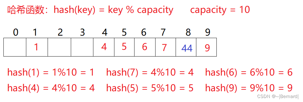
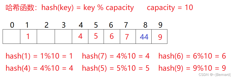
例如：数据集合{1，7，6，4，5，9}；
哈希函数设置为：hash(key) = key(关键码) % capacity; capacity为存储元素底层空间总的大小。

用该方法进行搜索不必进行多次关键码的比较，因此搜索的速度比较快

但是上面所给的数据求模过后都比较理想，如果按照上述哈希方式，再向集合中插入元素44，会出现什么问题呢？

2.2 哈希冲突

对于两个数据元素的关键字key1和key2，有 key1!=key2 ，但有：Hash( key1) == Hash(key2 )，即：不同关键字通过相同哈希函数计算出相同的哈希地址，该种现象称为哈希冲突或哈希碰撞。
把具有不同关键码而具有相同哈希地址的数据元素称为“同义词”。
那么发生哈希冲突又该如何处理呢？我们下面给出答案

2.3 哈希函数

引起哈希冲突的一个原因可能是：哈希函数设计不够合理。

哈希函数设计原则：
·哈希函数的定义域必须包括需要存储的全部关键码，而如果散列表允许有m个地址时，其值域必须在0到m-1之间
·哈希函数计算出来的地址能均匀分布在整个空间中
·哈希函数应该比较简单

下面给出几种常见的哈希函数：
1. 直接定址法--(常用)
取关键字的某个线性函数为散列地址：Hash（Key）= A*Key + B

优点：简单、均匀，适用于整数且数据范围比较集中，如果数据非常集中的话搜索速度快且节省空间每个值都对应一个唯一的位置,查找的时间复杂度为O(1)

缺点：需要事先知道关键字的分布情况,如果一组数据范围分部很大，直接定址法会浪费大量的空间，并且直接定址法不能处理字符串，浮点数这样的数据，使用场景很局限.

使用场景：适合查找比较小且连续的情况

给出一个直接定址法使用的例子：

力扣https://leetcode.cn/problems/first-unique-character-in-a-string/

class Solution {
public:
    int firstUniqChar(string s) 
    {
        int arr[26]={0};//创建一个数组来代表26个字符所对应位置字符出现的次数
        for(int i=0;i<s.size();i++)
        {
            arr[s[i]-'a']++;//相对映射的关系
        }
        for(int i=0;i<s.size();i++)
        {
            if(arr[s[i]-'a']==1)
            return i;
        }
        return -1;
    }
};

2. 除留余数法--(常用)
设散列表中允许的地址数为m，取一个不大于m，但最接近或者等于m的质数p作为除数，按照哈希函数：Hash(key) = key% p(p<=m),将关键码转换成哈希地址

优点：适用于数据范围很大的数，相对于直接定址法空间利用率很高，不会浪费太多空间

缺点： 不同的值会映射到同一个位置上，这样会造成哈希冲突.

3. 平方取中法--(不常用)
假设关键字为1234，对它平方就是1522756，抽取中间的3位227作为哈希地址； 再比如关键字为4321，对它平方就是18671041，抽取中间的3位671(或710)作为哈希地址 平方取中法比较适合：不知道关键字的分布，而位数又不是很大的情况

注意：哈希函数设计的越精妙，产生哈希冲突的可能性就越低，但是无法避免哈希冲突

2.4 哈希冲突解决

解决哈希冲突两种常见的方法是：闭散列和开散列

2.4.1 闭散列

闭散列：也叫开放定址法，当发生哈希冲突时，如果哈希表未被装满，说明在哈希表中必然还有空位置，那么可以把key存放到冲突位置中的“下一个” 空位置中去。用通俗的话来说，就是给冲突的值寻找新的位置.那如何寻找下一个空位置应该如何去找呢？

1. 线性探测Hash(key)=key%len+i (i=0,1,2,3...)
比如2.1中的场景，现在需要插入元素44，先通过哈希函数计算哈希地址，44%10=4，因此44理论上应该插在该4位置，但是该位置已经放了值为4的元素，即发生哈希冲突。
线性探测：从发生冲突的位置开始，依次向后探测，直到寻找到下一个空位置为止。

·插入
1.通过哈希函数获取待插入元素在哈希表中的位置

2.如果该位置中没有元素则直接插入新元素，如果该位置中有元素发生哈希冲突，使用线性探测找到下一个空位置，插入新元素

拿上面的44举例，44就应该往后找空位，则应该放入8这个空位置.

·删除
采用闭散列处理哈希冲突时，不能随便物理删除哈希表中已有的元素，若直接删除元素会影响其他元素的搜索。比如删除元素4，如果直接删除掉，44查找起来可能会受影响(因为如果删除4这个位置的值，查找44的时候会根据哈希函数先查找4这个位置，如果4为空了就不会再往后继续查找，所以44就不知道是否存在这个哈希表中，存在误判)。因此线性探测采用标记的伪删除法来删除一个元素。

下面给出线性探测的实现：

#pragma once
#include<iostream>
#include<string>
#include<vector>
using namespace std;


enum State
{
	EMPTY,//空标志
	DELETE,//删除标志
	EXIST//存在标志
};
template<class K,class V>
struct HashNode
{
	pair<K, V> _kv;
	State _s = EMPTY;
	//这里使用默认的构造函数就可以了
};
template<class K>
struct Hash
{
	size_t operator()(const K& key)
	{
		return key;
	}
};
// 特化
template<>
struct Hash<string>
{
	// "int"  "insert" 
	// 字符串转成对应一个整形值，因为整形才能取模算映射位置
	// 期望->字符串不同，转出的整形值尽量不同
	// "abcd" "bcad"
	// "abbb" "abca"
	size_t operator()(const string& s)
	{
		// BKDR Hash
		size_t value = 0;
		for (auto ch : s)
		{
			value += ch;
			value *= 131;
		}
		return value;
	}
};
template<class K, class V, class HashFunc = Hash<K>>
class HashTable
{
public:
	HashNode<K, V>* Find(const K& key)
	{
		if (_table.size() == 0)
		{
			return nullptr;
		}
		HashFunc hf;
		size_t start = hf(key) % _table.size();
		size_t index = start;
		size_t i = 1;
		while (_table[index]._s != EMPTY)//为空时就一直循环找空位
		{
			if (_table[index]._s == EXIST && _table[index]._kv.first == key)
			{
				return &_table[index];//返回这个地址
			}
			index = start + i;
			//二次探测：index=start+i*i;即可
			index %= _table.size();//防止走出数组
			i++;
		}
		return nullptr;
	}
	bool insert(const pair<K, V>& kv)
	{
		HashNode<K, V>* ret = Find(kv.first);
		if (ret)
		{
			//如果ret不为空，说明需要插入的元素已经在有了，就不可以插入
			return false;
		}

		if (_table.size() == 0)//刚开始容量为0时
		{
			_table.resize(10);//初始化给10个大小的空间
		}
		//负载因子大于0.7就增容
		//负载因子：存储有效数据格式/空间大小
		//负载因子越大，空间利用率越高，但是冲突概率越大，增删查改效率就越低
		//负载因子越小，空间利用率越小，但是冲突概率越小，增删查改效率越低
		else if ((double)_n /(double) _table.size() > 0.7)
		{
			HashTable<K, V, HashFunc> newHT;//创建一个新的哈希表
			newHT._table.resize(_table.size() * 2);//进行扩容
			for (auto& e : _table)//遍历原数组
			{
				if (e._s == EXIST)//如果状态为存在那么就插入到新的哈希表中
				{
					newHT.insert(e._kv);
				}
			}
			_table.swap(newHT._table);//最后交换一下vector即可
		}
		HashFunc hf;
		size_t start = hf(kv.first) % _table.size();
		size_t index = start;
		size_t i = 1;
		while (_table[index]._s == EXIST)//如果位置有其他值那么一直去找状态存在的那个空位
		{
			index = start + i;
			index %= _table.size();//防止走出数组
			++i;
		}
		_table[index]._kv = kv;//在这个位置插入数据
		_table[index]._s = EXIST;//把标志位置为存在
		++_n;//有效数据个数加一个
		return true;
	}
	bool Erase(const K& key)
	{
		HashNode<K, V>* ret = Find(key);
		if (ret == nullptr)
		{
			return false;
		}
		else
		{
			ret->_s = DELETE;
			return true;
		}
	}
private:
	vector<HashNode<K,V>> _table;//用一个vector来存储每一个节点
	size_t _n = 0;//存储有效数据的个数,默认初始给0
};

线性探测的代码测试：

#include"HashTable.h"



void TestHashTable1()
{
	int a[] = { 1, 5, 10, 100000, 100, 18, 15, 7, 40 };
	HashTable<int, int> ht;
	for (auto e : a)
	{
		ht.insert(make_pair(e, e));
	}
	auto ret = ht.Find(100);
	if (ret)
	{
		cout << "找到了" << endl;
	}
	else
	{
		cout << "没有找到" << endl;
	}

	ht.Erase(100);

	ret = ht.Find(100);
	if (ret)
	{
		cout << "找到了" << endl;
	}
	else
	{
		cout << "没有找到" << endl;
	}
}
void TestHashTable2()
{
	string a[] = { "苹果", "西瓜", "苹果", "西瓜", "苹果", "橘子", "苹果" };
	HashTable<string, int> ht;
 	for (auto str : a)
	{
		auto ret = ht.Find(str);
		if (ret)
		{
			ret->_kv.second++;
		}
		else
		{
			ht.insert(make_pair(str, 1));
		}
	}
}
struct stringHashFunc
{
	// "int"  "insert" 
	// 字符串转成对应一个整形值，因为整形才能取模算映射位置
	// 期望->字符串不同，转出的整形值尽量不同
	// "abcd" "bcad"
	// "abbb" "abca"
	size_t operator()(const string& s)
	{
		// BKDR Hash
		size_t value = 0;
		for (auto ch : s)
		{
			value += ch;
			value *= 131;
		}

		return value;
	}
};
void TestStringHashFunc()
{
	stringHashFunc hf;
	cout << hf("insert") << endl;
	cout << hf("int") << endl << endl;

	cout << hf("abcd") << endl;
	cout << hf("bacd") << endl << endl;

	cout << hf("abbb") << endl;
	cout << hf("abca") << endl << endl;
}

线性探测优点：实现非常简单，
线性探测缺点：一旦发生哈希冲突，所有的冲突连在一起，容易产生数据“堆积”，即：不同关键码占据了可利用的空位置，使得寻找某关键码的位置需要许多次比较，导致搜索效率降低。如何缓解呢？

2. 二次探测
线性探测的缺陷是产生冲突的数据堆积在一块，这与其找下一个空位置有关系，因为找空位置的方式就是挨着往后逐个去找，因此二次探测为了避免该问题每一次向后加平方次.

如果是二次探测只需要修改其中的部分细节

 研究表明：当表的长度为质数且表负载因子a不超过0.5时，新的表项一定能够插入，而且任何一个位置都不会被探查两次。因此只要表中有一半的空位置，就不会存在表满的问题。在搜索时可以不考虑表装满的情况，但在插入时必须确保表的装载因子a不超过0.5，如果超出必须考虑增容。

因此：闭散列最大的缺陷就是空间利用率比较低，这也是哈希的缺陷。

2.4.2 开散列

1. 开散列概念
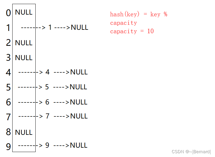
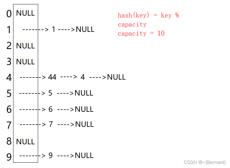
开散列法又叫链地址法(开链法)，首先对关键码集合用散列函数计算散列地址，具有相同地址的关键码归于同一子集合，每一个子集合称为一个桶，各个桶中的元素通过一个单链表链接起来，各链表的头结点存储在哈希表中。

从上图可以看出，开散列中每个桶中放的都是发生哈希冲突的元素。 

2. 开散列实现

template<class K,class V>
struct HashNode//定义哈希节点
{
	HashNode<K,V>* _next;
	pair<K, V> _kv;
	HashNode(const pair<K,V>& kv)
		:_next(nullptr)
		,_kv(kv)
	{}
};
template<class K>
struct Hash
{
	size_t operator()(const K& key)//仿函数
	{
		return key;
	}
};
// 特化
template<>
struct Hash < string >
{
	// "int"  "insert" 
	// 字符串转成对应一个整形值，因为整形才能取模算映射位置
	// 期望->字符串不同，转出的整形值尽量不同
	// "abcd" "bcad"
	// "abbb" "abca"
	size_t operator()(const string& s)//仿函数
	{
		// BKDR Hash
		size_t value = 0;
		for (auto ch : s)
		{
			value += ch;
			value *= 131;
		}

		return value;
	}
};
template<class K, class V, class HashFunc = Hash<K>>
class HashTable
{
	typedef HashNode<K, V> Node;
public:
	Node* Find(const K& key)
	{
		if (_table.size() == 0)//如果表的大小为0那么返回空
		{
			return nullptr;
		}
		HashFunc hf;//定义反函数对象
		size_t index = hf(key) % _table.size();//计算在表中的位置
		Node* cur = _table[index];//
		while (cur)//循环去找这个cur的节点
		{
			if (cur->_kv.first == key)
			{
				return cur;
			}
			else
			{
				cur = cur->_next;
			}
		}
		return nullptr;
	}
	bool Insert(const pair<K,V>& kv)
	{
		Node* ret = Find(kv.first);//先进行查找
		if (ret)//如果查找的节点不为空，说明数据在表中存在，而我们不允许数据冗余，故返回错误
		{
			return false;
		}

		HashFunc hf;//定义仿函数对象
		if (_n == _table.size())//如果为空或者有效数据个数达到数组容量则需要扩容
		{
			//开散列最好的情况是：每个哈希桶中刚好挂一个节点，再继续插入元素时，每一次都会发
			//生哈希冲突，因此，在元素个数刚好等于桶的个数时，可以给哈希表增容。
			vector<Node*> newTable;
			size_t newsize = _table.size() == 0 ? 8 : _table.size() * 2;
			newTable.resize(newsize, nullptr);

			for (size_t i = 0; i < _table.size(); i++)//对扩容的数据转移到新的vector中
			{
				if (_table[i])//如果这个位置不为空那么则需要进行数据的挪动
				{
					Node* cur = _table[i];//进入循环之前记录一下cur节点
					while (cur)//循环去挪动每一个不为空的节点
					{
						size_t index = hf(cur->_kv.first) % newsize;//每一次都需要计算一下索引位置
						Node* next = cur->_next;//需要记录一下

						//头插
						cur->_next = newTable[index];
						newTable[index] = cur;

						cur = next;
					}
					_table[i] = nullptr;
				}
			}
			_table.swap(newTable);//最后进行一下交换
		}
		//如果不需要增容时:
		size_t index = hf(kv.first) % _table.size();
		Node* newnode = new Node(kv);
		//进行头插
		newnode->_next = _table[index];
		_table[index] = newnode;
		++_n;//有效数据个数加一

		return true;
	}
	//删除法一：边查找边删除
	/*bool Erase(const K& key)
	{
		HashFunc hf;
		size_t index = hf(key) % _table.size();
		Node* prev = nullptr;
		Node* cur = _table[index];
		while (cur)
		{
			if (cur->_kv.first == key)
			{
				if (cur == _table[index])
				{
					_table[index] = cur->_next;
				}
				else
				{
					prev->_next = cur->_next;
				}
				delete cur;
				--_n;
				return true;
			}
			else
			{
				prev = cur;
				cur = cur->_next;
			}
		}
		return false;
	}*/
	//删除法二：替代法删除：替代法删除的好处就是不需要指针prev，在没有办法找到前一个指针的时候，采用替代法删除是一个很好的思路
	bool Erase(const K& key)
	{
		HashFunc hf;

		Node* ret = Find(key);//先用查找算法找到该节点
		if (ret == nullptr)//节点为空则返回false
		{
			return false;
		}
		else//不为空就要进行删除操作
		{
			size_t index = hf(key) % _table.size();//计算出在数组中的位置
			if (ret == _table[index])//如果删除的节点就是这个位置的节点
			{
				delete ret;
				--_n;
				_table[index] = nullptr;
				return true;
			}
			else
			{
				Node* next = ret->_next;//用next记录下一个节点
				if (next)//如果下一个节点不为空就删除下一个节点，并且提前把值给ret
				{
					ret->_kv = next->_kv;
					ret->_next = next->_next;
					delete next;
					--_n;
				}
				else
				{
					//下一个节点为空就转换为删除第一个节点，并且提前把值给ret
					Node* begin = _table[index];
					ret->_kv = begin->_kv;
					_table[index] = begin->_next;
					delete begin;
					--_n;
				}
				return true;
			}
			return false;
		}
	}
private:
	vector<Node*> _table;
	size_t _n;
};

开散列模拟实现测试：

void TestHashTable1()
{
	int a[] = { 1, 5, 10, 100000, 100, 18, 15, 7, 40,26 };
	HashTable<int, int> ht;
	for (auto e : a)
	{
		ht.Insert(make_pair(e, e));
	}
	auto ret = ht.Find(100);
	if (ret)
	{
		cout << "找到了" << endl;
	}
	else
	{
		cout << "没有找到" << endl;
	}

	ht.Erase(100);

	ret = ht.Find(100);
	if (ret)
	{
		cout << "找到了" << endl;
	}
	else
	{
		cout << "没有找到" << endl;
	}

	ht.Erase(10);
	ret = ht.Find(10);
	if (ret)
	{
		cout << "找到了" << endl;
	}
	else
	{
		cout << "没有找到" << endl;
	}
}

3. 模拟实现

3.1 哈希表的改造

1. 模板参数列表的改造

// K:关键码类型
// T: 不同容器T的类型不同，如果是unordered_map，T代表一个键值对，如果是unordered_set,T为 K
// KeyOfT: 因为T的类型不同，通过T取key的方式就不同，详细见unordered_map/set的实现
// HashFunc: 哈希函数仿函数对象类型，哈希函数使用除留余数法，需要将Key转换为整形数字才能取模
template<class K, class T, class KeyOfT, class HashFunc = Hash<K>>
class HashTable;

2. 增加迭代器操作

// 迭代器
template<class K, class T, class KeyOfT, class HashFunc = Hash<K>>
struct __HTIterator
{
	typedef HashNode<T> Node;
	typedef __HTIterator<K, T, KeyOfT, HashFunc> Self;
	typedef HashTable<K, T, KeyOfT, HashFunc> HT;
	Node* _node;
	HT* _pht;//需要一个哈希表指针(实际也就是vector数组)

	__HTIterator(Node* node, HT* pht)//迭代器指针
		:_node(node)
		, _pht(pht)
	{}

	Self& operator++()
	{
		if (_node->_next)// 1、当前桶中不为空也就是还有数据，那么就在当前桶往后走
		{
			_node = _node->_next;
		}
		else// 2、当前桶走完了，需要往下一个桶去走。
		{
			//size_t index = HashFunc()(KeyOfT()(_node->_data)) % _pht->_table.size();
			KeyOfT kot;//仿函数对象kot，用以取其中的T数据
			HashFunc hf;//用以取key数据
			size_t index = hf(kot(_node->_data)) % _pht->_table.size();

			++index;
			while (index < _pht->_table.size())//索引值小于表大小时就一直循环找
			{
				if (_pht->_table[index])//如果不为空，那么就把node指向这个表对应位置的元素
				{
					_node = _pht->_table[index];
					return *this;//返回this指针
				}
				else//为空就需要++往后迭代
				{
					++index;
				}
			}
			_node = nullptr;//这一步操作是当表走完的时候将这个节点置空
		}
		return *this;
	}
	T& operator*()
	{
		return _node->_data;
	}
	T* operator->()
	{
		return &_node->_data;
	}
	bool operator != (const Self& s) const
	{
		return _node != s._node;
	}
	bool operator == (const Self& s) const
	{
		return _node == s.node;
	}
};

3. 重新增加迭代器功能后对模拟实现进行进一步改写：
 

template<class K>
struct Hash
{
	size_t operator()(const K& key)
	{
		return key;
	}
};
// 特化
template<>
struct Hash < string >
{
	// "int"  "insert" 
	// 字符串转成对应一个整形值，因为整形才能取模算映射位置
	// 期望->字符串不同，转出的整形值尽量不同
	// "abcd" "bcad"
	// "abbb" "abca"
	size_t operator()(const string& s)
	{
		// BKDR Hash
		size_t value = 0;
		for (auto ch : s)
		{
			value += ch;
			value *= 131;
		}

		return value;
	}
};
template<class T>
struct HashNode
{
	HashNode<T>* _next;
	T _data;

	HashNode(const T& data)
		:_next(nullptr)
		, _data(data)
	{}
};
// 前置声明
template<class K, class T, class KeyOfT, class HashFunc>
class HashTable;
// 迭代器
template<class K, class T, class KeyOfT, class HashFunc = Hash<K>>
struct __HTIterator
{
	typedef HashNode<T> Node;
	typedef __HTIterator<K, T, KeyOfT, HashFunc> Self;
	typedef HashTable<K, T, KeyOfT, HashFunc> HT;
	Node* _node;
	HT* _pht;//需要一个哈希表指针(实际也就是vector数组)

	__HTIterator(Node* node, HT* pht)//迭代器指针
		:_node(node)
		, _pht(pht)
	{}

	Self& operator++()
	{
		if (_node->_next)// 1、当前桶中不为空也就是还有数据，那么就在当前桶往后走
		{
			_node = _node->_next;
		}
		else// 2、当前桶走完了，需要往下一个桶去走。
		{
			//size_t index = HashFunc()(KeyOfT()(_node->_data)) % _pht->_table.size();
			KeyOfT kot;//仿函数对象kot，用以取其中的T数据
			HashFunc hf;//用以取key数据
			size_t index = hf(kot(_node->_data)) % _pht->_table.size();

			++index;
			while (index < _pht->_table.size())//索引值小于表大小时就一直循环找
			{
				if (_pht->_table[index])//如果不为空，那么就把node指向这个表对应位置的元素
				{
					_node = _pht->_table[index];
					return *this;//返回this指针
				}
				else//为空就需要++往后迭代
				{
					++index;
				}
			}
			_node = nullptr;//这一步操作是当表走完的时候将这个节点置空
		}
		return *this;
	}
	T& operator*()
	{
		return _node->_data;
	}
	T* operator->()
	{
		return &_node->_data;
	}
	bool operator != (const Self& s) const
	{
		return _node != s._node;
	}
	bool operator == (const Self& s) const
	{
		return _node == s.node;
	}
};
template<class K, class T, class KeyOfT, class HashFunc = Hash<K>>
class HashTable
{
	typedef HashNode<T> Node;

	template<class K, class T, class KeyOfT, class HashFunc>
	friend struct __HTIterator;//定义友元类

public:
	typedef __HTIterator<K, T, KeyOfT, HashFunc> iterator;

	HashTable() = default; // 显示指定生成默认构造

	HashTable(const HashTable& ht)//自定义拷贝构造
	{
		_n = ht._n;
		_table.resize(ht._table.size());
		for (size_t i = 0; i < ht._table.size(); i++)
		{
			Node* cur = ht._table[i];
			while (cur)
			{
				Node* copy = new Node(cur->_data);
				// 头插到新表
				copy->_next = _table[i];
				_table[i] = copy;

				cur = cur->_next;
			}
		}
	}
	HashTable& operator=(HashTable ht)//赋值拷贝
	{
		_table.swap(ht._table);
		swap(_n, ht._n);

		return *this;
	}
	~HashTable()//析构函数
	{
		for (size_t i = 0; i < _table.size(); ++i)
		{
			Node* cur = _table[i];
			while (cur)
			{
				Node* next = cur->_next;
				delete cur;
				cur = next;
			}
			_table[i] = nullptr;
		}
	}
	iterator begin()
	{
		size_t i = 0;
		while (i < _table.size())//循环去找表中不为空的那个位置
		{
			if (_table[i])//如果不为空那么返回这个位置用迭代器封装的指针
			{
				return iterator(_table[i], this);//传this指针是因为需要找到这个表
			}
			++i;//否则进行++
		}
		return end();//如果循环结束还没有找到那么久返回nullptr
	}
	iterator end()
	{
		return iterator(nullptr, this);
	}
	//除留余数法，最好模一个素数，每次快速取一个类似两倍关系的素数
	size_t GetNextPrime(size_t prime)
	{
		const int PRIMECOUNT = 28;
		static const size_t primeList[PRIMECOUNT] =
		{
			53ul, 97ul, 193ul, 389ul, 769ul,
			1543ul, 3079ul, 6151ul, 12289ul, 24593ul,
			49157ul, 98317ul, 196613ul, 393241ul, 786433ul,
			1572869ul, 3145739ul, 6291469ul, 12582917ul, 25165843ul,
			50331653ul, 100663319ul, 201326611ul, 402653189ul, 805306457ul,
			1610612741ul, 3221225473ul, 4294967291ul
		};
		size_t i = 0;
		for (; i < PRIMECOUNT; ++i)
		{
			if (primeList[i] > prime)
				return primeList[i];
		}
		return primeList[i];
	}
	pair<iterator, bool> Insert(const T& data)
	{
		KeyOfT kot;
		// 找到了
		auto ret = Find(kot(data));
		if (ret != end())
			return make_pair(ret, false);

		HashFunc hf;
		// 负载因子到1时，进行增容
		if (_n == _table.size())
		{
			vector<Node*> newtable;
			newtable.resize(GetNextPrime(_table.size()));

			// 遍历取旧表中节点，重新算映射到新表中的位置，挂到新表中
			for (size_t i = 0; i < _table.size(); ++i)
			{
				if (_table[i])
				{
					Node* cur = _table[i];
					while (cur)
					{
						Node* next = cur->_next;
						size_t index = hf(kot(cur->_data)) % newtable.size();
						// 头插
						cur->_next = newtable[index];
						newtable[index] = cur;

						cur = next;
					}
					_table[i] = nullptr;
				}
			}

			_table.swap(newtable);
		}

		size_t index = hf(kot(data)) % _table.size();
		Node* newnode = new Node(data);

		// 头插
		newnode->_next = _table[index];
		_table[index] = newnode;
		++_n;

		return make_pair(iterator(newnode, this), true);
	}

	iterator Find(const K& key)
	{
		if (_table.size() == 0)
		{
			return end();
		}

		KeyOfT kot;
		HashFunc hf;
		size_t index = hf(key) % _table.size();
		Node* cur = _table[index];
		while (cur)
		{
			if (kot(cur->_data) == key)
			{
				return iterator(cur, this);
			}
			else
			{
				cur = cur->_next;
			}
		}

		return end();
	}
	bool Erase(const K& key)
	{
		size_t index = hf(key) % _table.size();
		Node* prev = nullptr;
		Node* cur = _table[index];
		while (cur)
		{
			if (kot(cur->_data) == key)
			{
				if (_table[index] == cur)
				{
					_table[index] = cur->_next;
				}
				else
				{
					prev->_next = cur->_next;
				}

				--_n;
				delete cur;
				return true;
			}

			prev = cur;
			cur = cur->_next;
		}

		return false;
	}
private:
	vector<Node*> _table;
	size_t _n = 0;         // 有效数据的个数
};

3.2 unordered_map的封装和模拟实现代码测试

template<class K, class V>
class unordered_map
{
	struct MapKeyOfT
	{
		const K& operator()(const pair<K, V>& kv)//map里面存放的键值对
		{
			return kv.first;//返回键值对中的K
		}
	};
public:
	typedef typename HashTable<K, pair<K, V>, MapKeyOfT>::iterator iterator;
	iterator begin()
	{
		return _ht.begin();
	}
	iterator end()
	{
		return _ht.end();
	}
	pair<iterator, bool> insert(const pair<K, V>& kv)
	{
		return _ht.Insert(kv);
	}
	V& operator[](const K& key)//重载operator[]
	{
		pair<iterator, bool> ret = _ht.Insert(make_pair(key, V()));
		return ret.first->second;
	}
private:
	HashTable<K, pair<K, V>, MapKeyOfT> _ht;
};
void test_unordered_map1()
{
	unordered_map<string, string> dict;
	dict.insert(make_pair("sort", ""));
	dict["left"] = "";
	dict["left"] = "左边";
	dict["map"] = "地图";
	dict["string"] = "字符串";
	dict["set"] = "设置";

	unordered_map<string, string>::iterator it = dict.begin();
	while (it != dict.end())
	{
		cout << it->first << ":" << it->second << endl;
		++it;
	}
	cout << endl;
}

3.2 unordered_set的封装和模拟实现代码测试

template<class K>
class unordered_set
{
	struct SetKeyOfT
	{
		const K& operator()(const K& k)
		{
			return k;
		}
	};
public:
	typedef typename HashTable<K, K, SetKeyOfT >::iterator iterator;//加typename是为了告诉编译器在未实例化之前去找
	iterator begin()
	{
		return _ht.begin();
	}
	iterator end()
	{
		return _ht.end();
	}
	pair<iterator, bool> insert(const K k)
	{
		return _ht.Insert(k);
	}
private:
	HashTable<K, K, SetKeyOfT> _ht;
};
void test_unordered_set1()
{
	unordered_set<int> us;
	us.insert(200);
	us.insert(1);
	us.insert(2);
	us.insert(33);
	us.insert(50);
	us.insert(60);
	us.insert(243);
	us.insert(6);

	unordered_set<int>::iterator it = us.begin();
	while (it != us.end())
	{
		cout << *it << " ";
		++it;
	}
}

开散列与闭散列比较
应用链地址法(开散列)处理溢出，需要增设链接指针，似乎增加了存储开销。事实上： 由于闭散列必须保持大量的空闲空间以确保搜索效率，如二次探查法要求装载因子a <= 0.7，而表项所占空间又比指针大的多，所以使用链地址法(开散列)反而比闭散列节省存储空间