


目录
已多次训练的模型文件 73%(放置在.py同目录下)(第一种模型)
过拟合程度较低的模型文件70%(放置在.py同目录下)(第一种模型)
实验内容:
使用pytorch对cifar10进行分类。
代码流程:
- 定义网络
- CIFAR-10的下载及录入。
- 数据预处理
- 模型加载
- 训练模型
- 测试模型
- 绘制图像
Cifar-10及模型文件下载:
如果嫌自动下载太慢 :cifar-10下载
cifa-10解压后,将 cifar-10-batches-py放置在 .py 文件同目录下的 dataset 文件夹
Cifar-10及已训练模型(cnn.pth)放置位置如图:


已多次训练的模型文件 73%(放置在.py同目录下)(第一种模型)
这个过拟合了,如果需要更高的准确率,可以尝试重新训练,
如果欠拟合,可以尝试更改模型,增加训练次数,重新训练旧有模型(推荐)等。
如果更改模型,旧有模型文件将无法使用(不过训练的挺快的。)
过拟合程度较低的模型文件70%(放置在.py同目录下)(第一种模型)

已多次训练的模型文件 66%(放置在.py同目录下)(第二种模型)
全部代码:
8轮训练约6min
减少卷积层和全连接层能够更快的训练
看着挺密集,注释挺多的,应该好理解。
import torchvision as tv # 专门用来处理图像的库
from torchvision import transforms # transforms用来对图片进行变换
from torchvision.transforms import ToPILImage
import os # 用于加载旧模型使用
import torch
import torch.nn as nn # 神经网络基本工具箱
import torch.nn.functional as fun
import numpy as np
import matplotlib.pyplot as plt # 绘图模块,能绘制 2D 图表
# 定义卷积神经网络==========================================================
class ConvNet(nn.Module): # 类 ConvNet 继承自 nn.Module
def __init__(self): # 构造方法
# 下式等价于nn.Module.__init__.(self)
super(ConvNet, self).__init__() # 调用父类构造方法
# 使用了三个卷积层,四个全连接层
# RGB 3*32*32
# 卷积层===========================================================
self.conv1 = nn.Conv2d(3, 15, 3) # 输入3通道,输出15通道,卷积核为3*3
self.conv2 = nn.Conv2d(15, 75, 4) # 输入15通道,输出75通道,卷积核为4*4
self.conv3 = nn.Conv2d(75, 375, 3) # 输入75通道,输出375通道,卷积核为3*3
# 全连接层=========================================================
self.fc1 = nn.Linear(1500, 400) # 输入2000,输出400
self.fc2 = nn.Linear(400, 120) # 输入400,输出120
self.fc3 = nn.Linear(120, 84) # 输入120,输出84
self.fc4 = nn.Linear(84, 10) # 输入 84,输出 10(分10类)
def forward(self, x):
# 最大池化步长为2
x = fun.max_pool2d(fun.relu(self.conv1(x)), 2) # 3*32*32 -> 150*30*30 -> 15*15*15
x = fun.max_pool2d(fun.relu(self.conv2(x)), 2) # 15*15*15 -> 75*12*12 -> 75*6*6
x = fun.max_pool2d(fun.relu(self.conv3(x)), 2) # 75*6*6 -> 375*4*4 -> 375*2*2
x = x.view(x.size()[0], -1) # 将375*2*2的tensor打平成1维,(卷积变为全连接)1500
x = fun.relu(self.fc1(x)) # 全连接层 1500 -> 400
x = fun.relu(self.fc2(x)) # 全连接层 400 -> 120
x = fun.relu(self.fc3(x)) # 全连接层 120 -> 84
x = self.fc4(x) # 全连接层 84 -> 10
return x
# ==========================================================================================================
# 数据预处理
transform = transforms.Compose([
transforms.ToTensor(), # 将图片类型由 PIL Image 转化成tensor类型。转换时会自动归一化
transforms.Normalize((0.5, 0.5, 0.5), (0.5, 0.5, 0.5))]) # 对图像进行标准化(均值变为0,标准差变为1)
# 下载数据集==========================================
print("开始导入数据集==============================================")
classes = ('plane', 'car', 'bird', 'cat', 'deer', 'dog', 'frog', 'horse', 'ship', 'truck')
# 下载(download) cifar-10 后放到项目中的 dataset 文件夹(root)并分为训练集,测试集,(train)并做预处理(transform)
train_start = tv.datasets.CIFAR10(root="./dataset", train=True, download=True, transform=transform) # 训练集
test_set = tv.datasets.CIFAR10(root="./dataset", train=False, download=True, transform=transform) # 测试集
print('训练及图像有:', len(train_start), '张。\n测试集图像有:', len(test_set), '张。')
# 打包数据集 python将多个数据打包处理,能够加快训练速度
batch_size = 4
# 将测试集和训练集每 4个 进行打包,并打乱训练集(shuffle)
train_set = torch.utils.data.DataLoader(train_start, batch_size=batch_size, shuffle=True) # 训练集
test_set = torch.utils.data.DataLoader(test_set, batch_size=batch_size, shuffle=False) # 测试集
# 设置卷积神经网络和训练参数=================================
print("正在加载卷积神经网络=========================================")
# 如果设备 GPU 能被调用,则转到 GPU 加快运算,否则使用CPU
device = torch.device('cuda' if torch.cuda.is_available() else 'cpu')
model = ConvNet().to(device) # 初始化模型
print(device)
print('可使用GPU加速' if (torch.cuda.is_available()) else '无法开启GPU加速')
learning_rate = 0.001 # 学习率
criterion = nn.CrossEntropyLoss() # 交叉熵损失函数
optimizer = torch.optim.SGD(model.parameters(), lr=learning_rate) # 优化器:随机梯度下降算法
loop = 8 # 循环次数
print("学习率为", learning_rate, "\n训练次数为:", loop)
# 模型加载==========================================
i = 0 # 绘图用
seat = './cnn.pth' # 保存位置(名称)
if os.path.exists(seat): # 如果检测到 seat 文件
print("检测到模型文件,是否加载已训练模型(Y\\N):")
shuru = input()
if shuru == 'Y' or shuru == 'y':
model.load_state_dict(torch.load(seat))
print("已加载已训练模型")
print("是否继续训练(Y\\N):")
shuru = input() # 加载模型用户决定是否训练
else:
print("未加载已训练模型")
shuru = 'Y' # 不加载模型直接训练
else:
print("未检测到旧模型文件")
shuru = 'Y' # 不加载模型直接训练
# 开始训练==========================================
if shuru == 'Y' or shuru == 'y':
print("开始训练===================================================")
print("训练结果会自动保存")
lentrain = len(train_set)
process = []
for epoch in range(loop): # 训练 loop 次
running_loss = 0.0 # 训练误差
# 下面这个作用是每轮打乱一次,没什么大用处,不想要可以删去
train_set = torch.utils.data.DataLoader(train_start, batch_size=batch_size, shuffle=True) # 训练集
# enumerate() 函数:用于将一个可遍历的数据对象(如列表、元组或字符串)组合为一个索引序列,同时列出数据和数据下标。
for i, (images, labels) in enumerate(train_set, 0):
# 转到GPU或CPU上进行运算
images = images.to(device)
labels = labels.to(device)
outputs = model(images) # 正向传播
loss = criterion(outputs, labels) # 计算batch(四个一打包)误差
optimizer.zero_grad() # 梯度清零
loss.backward() # 反向传播
optimizer.step() # 更新参数
# 打印loss信息
running_loss += loss.item() # 2000个batch的误差和
if i % 2000 == 1999: # 每2000个batch打印一次训练状态
print("第%2d/%2d 轮循环,%6d/%6d 组,误差为:%.4f"
% (epoch + 1, loop, i + 1, lentrain, running_loss / 2000))
process.append(running_loss)
running_loss = 0.0 # 误差归零
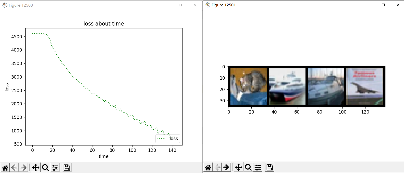
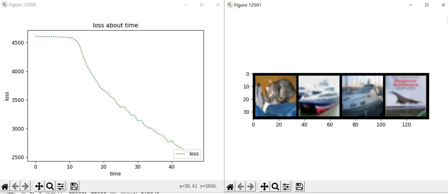
# 绘制训练过程
i = i + 1
plt.figure(i)
plt.plot(list(range(len(process))), process, 'g:', label='loss')
plt.legend(loc='lower right') # 显示上面的label
plt.xlabel('time') # x_label
plt.ylabel('loss') # y_label
plt.title('loss about time') # 标题
# 模型保存==========================================
print("保存模型至%s======================================" % seat)
torch.save(model.state_dict(), seat)
print("保存完毕")
# 模型测试==========================================
print("开始测试===================================================")
# 在训练集上测试====================================
correct = 0 # 预测正确图片数
total = 0 # 总图片数
for images, labels in train_set:
images = images.to(device)
labels = labels.to(device)
outputs = model(images)
# 返回得分最高的索引(一组 4 个)
_, predicted = torch.max(outputs.data, 1)
total += labels.size(0)
correct += (predicted == labels).sum()
print("训练集中的准确率为:%d %%" % (100 * correct / total))
# 在测试集上测试====================================
correct = 0 # 预测正确图片数
total = 0 # 总图片数
for images, labels in test_set:
images = images.to(device)
labels = labels.to(device)
outputs = model(images)
# 返回得分最高的索引(一组 4 个)
_, predicted = torch.max(outputs.data, 1)
total += labels.size(0)
correct += (predicted == labels).sum()
print("测试集中的准确率为:%d %%" % (100 * correct / total))
# 输出在测试集上一组(4个)的数据和预测结果===================
dataiter = iter(test_set) # 生成测试集的可迭代对象
images, labels = dataiter.next() # 得到一组数据
# 绘图====================
i = i + 1
plt.figure(i)
npimg = (tv.utils.make_grid(images / 2 + 0.5)).numpy()
plt.imshow(np.transpose(npimg, (1, 2, 0)))
print("实际标签:", " ".join("%08s" % classes[labels[j]] for j in range(4)))
show = ToPILImage() # 把tensor转为image
images = images.to(device)
labels = labels.to(device)
outputs = model(images) # 计算图片在每个类别上的分数
# 返回得分最高的索引
_, predicted = torch.max(outputs.data, 1) # 第一个数是具体值,不需要
# 一组 4 张图,所以找每行的最大值
print("预测结果:", " ".join("%08s" % classes[predicted[j]] for j in range(4)))
plt.show() # 显示=========
训练结果:
3层卷积层和池化层,4层全连接层。最大池化层步长为2。
第一种模型:
代码如下:
8轮训练约 6 分钟训练集测试集正确率可达50+%
如果你的时间比较多,可以不打包(把打包数改为1)也能提升准确率
如果loss图像不再呈下降趋势,可以减少学习率,继续训练。(注意过拟合)
# 定义卷积神经网络==========================================================
class ConvNet(nn.Module):  # 类 ConvNet 继承自 nn.Module
    def __init__(self):  # 构造方法
        # 下式等价于nn.Module.__init__.(self)
        super(ConvNet, self).__init__()  # 调用父类构造方法
        # 使用了三个卷积层,四个全连接层
        # RGB 3*32*32
        # 卷积层===========================================================
        self.conv1 = nn.Conv2d(3, 15, 3)  # 输入3通道,输出15通道,卷积核为3*3
        self.conv2 = nn.Conv2d(15, 75, 4)  # 输入15通道,输出75通道,卷积核为4*4
        self.conv3 = nn.Conv2d(75, 375, 3)  # 输入75通道,输出375通道,卷积核为3*3
        # 全连接层=========================================================
        self.fc1 = nn.Linear(1500, 400)  # 输入2000,输出400
        self.fc2 = nn.Linear(400, 120)  # 输入400,输出120
        self.fc3 = nn.Linear(120, 84)  # 输入120,输出84
        self.fc4 = nn.Linear(84, 10)  # 输入 84,输出 10(分10类)

    def forward(self, x):
        # 最大池化步长为2
        x = fun.max_pool2d(fun.relu(self.conv1(x)), 2)  # 3*32*32  -> 150*30*30  -> 15*15*15
        x = fun.max_pool2d(fun.relu(self.conv2(x)), 2)  # 15*15*15 -> 75*12*12  -> 75*6*6
        x = fun.max_pool2d(fun.relu(self.conv3(x)), 2)  # 75*6*6   -> 375*4*4   -> 375*2*2
        x = x.view(x.size()[0], -1)  # 将375*2*2的tensor打平成1维,(卷积变为全连接)1500
        x = fun.relu(self.fc1(x))  # 全连接层 1500 -> 400
        x = fun.relu(self.fc2(x))  # 全连接层 400 -> 120
        x = fun.relu(self.fc3(x))  # 全连接层 120 -> 84
        x = self.fc4(x)  # 全连接层 84  -> 10
        return x
训练过程:
开始导入数据集==============================================
Files already downloaded and verified
Files already downloaded and verified
训练及图像有: 50000 张。
测试集图像有: 10000 张。
正在加载卷积神经网络=========================================
cuda
可使用GPU加速
学习率为 0.001
训练次数为: 8
检测到模型文件,是否加载已训练模型(Y\N):
n
未加载已训练模型
开始训练===================================================
训练结果会自动保存
第 1/ 8 轮循环,  2000/ 12500 组,误差为:2.3039
第 1/ 8 轮循环,  4000/ 12500 组,误差为:2.3028
第 1/ 8 轮循环,  6000/ 12500 组,误差为:2.3023
第 1/ 8 轮循环,  8000/ 12500 组,误差为:2.3013
第 1/ 8 轮循环, 10000/ 12500 组,误差为:2.3012
第 1/ 8 轮循环, 12000/ 12500 组,误差为:2.3006
第 2/ 8 轮循环,  2000/ 12500 组,误差为:2.2995
第 2/ 8 轮循环,  4000/ 12500 组,误差为:2.2990
第 2/ 8 轮循环,  6000/ 12500 组,误差为:2.2972
第 2/ 8 轮循环,  8000/ 12500 组,误差为:2.2952
第 2/ 8 轮循环, 10000/ 12500 组,误差为:2.2919
第 2/ 8 轮循环, 12000/ 12500 组,误差为:2.2852
第 3/ 8 轮循环,  2000/ 12500 组,误差为:2.2652
第 3/ 8 轮循环,  4000/ 12500 组,误差为:2.2210
第 3/ 8 轮循环,  6000/ 12500 组,误差为:2.1317
第 3/ 8 轮循环,  8000/ 12500 组,误差为:2.0523
第 3/ 8 轮循环, 10000/ 12500 组,误差为:2.0022
第 3/ 8 轮循环, 12000/ 12500 组,误差为:1.9558
第 4/ 8 轮循环,  2000/ 12500 组,误差为:1.9096
第 4/ 8 轮循环,  4000/ 12500 组,误差为:1.8596
第 4/ 8 轮循环,  6000/ 12500 组,误差为:1.8319
第 4/ 8 轮循环,  8000/ 12500 组,误差为:1.8148
第 4/ 8 轮循环, 10000/ 12500 组,误差为:1.7812
第 4/ 8 轮循环, 12000/ 12500 组,误差为:1.7598
第 5/ 8 轮循环,  2000/ 12500 组,误差为:1.7161
第 5/ 8 轮循环,  4000/ 12500 组,误差为:1.6853
第 5/ 8 轮循环,  6000/ 12500 组,误差为:1.6911
第 5/ 8 轮循环,  8000/ 12500 组,误差为:1.6542
第 5/ 8 轮循环, 10000/ 12500 组,误差为:1.6195
第 5/ 8 轮循环, 12000/ 12500 组,误差为:1.6182
第 6/ 8 轮循环,  2000/ 12500 组,误差为:1.5706
第 6/ 8 轮循环,  4000/ 12500 组,误差为:1.5715
第 6/ 8 轮循环,  6000/ 12500 组,误差为:1.5304
第 6/ 8 轮循环,  8000/ 12500 组,误差为:1.5078
第 6/ 8 轮循环, 10000/ 12500 组,误差为:1.5062
第 6/ 8 轮循环, 12000/ 12500 组,误差为:1.4785
第 7/ 8 轮循环,  2000/ 12500 组,误差为:1.4556
第 7/ 8 轮循环,  4000/ 12500 组,误差为:1.4451
第 7/ 8 轮循环,  6000/ 12500 组,误差为:1.4233
第 7/ 8 轮循环,  8000/ 12500 组,误差为:1.3809
第 7/ 8 轮循环, 10000/ 12500 组,误差为:1.3972
第 7/ 8 轮循环, 12000/ 12500 组,误差为:1.3602
第 8/ 8 轮循环,  2000/ 12500 组,误差为:1.3418
第 8/ 8 轮循环,  4000/ 12500 组,误差为:1.3309
第 8/ 8 轮循环,  6000/ 12500 组,误差为:1.2963
第 8/ 8 轮循环,  8000/ 12500 组,误差为:1.3022
第 8/ 8 轮循环, 10000/ 12500 组,误差为:1.2693
第 8/ 8 轮循环, 12000/ 12500 组,误差为:1.2843
保存模型至./cnn.pth======================================
保存完毕
开始测试===================================================
训练集中的准确率为:55 %
测试集中的准确率为:54 %
实际标签:      cat     ship     ship    plane
预测结果:      cat     ship     ship     ship
第二种模型:
如果用以下卷积神经网络,8轮训练约 6分钟,可达50+%
class ConvNet(nn.Module):
    def __init__(self):
        super(ConvNet, self).__init__()
        self.conv1 = nn.Conv2d(3, 6, 5)
        self.pool = nn.MaxPool2d(2, 2)
        self.conv2 = nn.Conv2d(6, 16, 5)
        self.fc1 = nn.Linear(16 * 5 * 5, 120)
        self.fc2 = nn.Linear(120, 84)
        self.fc3 = nn.Linear(84, 10)

    def forward(self, x):
        x = self.pool(F.relu(self.conv1(x)))
        x = self.pool(F.relu(self.conv2(x)))
        x = x.view(-1, 16 * 5 * 5)
        x = F.relu(self.fc1(x))
        x = F.relu(self.fc2(x))
        x = self.fc3(x)
        return x
训练过程:
开始导入数据集==============================================
Files already downloaded and verified
Files already downloaded and verified
训练及图像有: 50000 张。
测试集图像有: 10000 张。
正在加载卷积神经网络=========================================
cuda
可使用GPU加速
学习率为 0.001
训练次数为: 8
未检测到旧模型文件
开始训练===================================================
训练结果会自动保存
第 1/ 8 轮循环,  2000/ 12500 组,误差为:2.3037
第 1/ 8 轮循环,  4000/ 12500 组,误差为:2.3005
第 1/ 8 轮循环,  6000/ 12500 组,误差为:2.2982
第 1/ 8 轮循环,  8000/ 12500 组,误差为:2.2896
第 1/ 8 轮循环, 10000/ 12500 组,误差为:2.2701
第 1/ 8 轮循环, 12000/ 12500 组,误差为:2.2173
第 2/ 8 轮循环,  2000/ 12500 组,误差为:2.1186
第 2/ 8 轮循环,  4000/ 12500 组,误差为:2.0516
第 2/ 8 轮循环,  6000/ 12500 组,误差为:1.9952
第 2/ 8 轮循环,  8000/ 12500 组,误差为:1.9494
第 2/ 8 轮循环, 10000/ 12500 组,误差为:1.8899
第 2/ 8 轮循环, 12000/ 12500 组,误差为:1.8465
第 3/ 8 轮循环,  2000/ 12500 组,误差为:1.7775
第 3/ 8 轮循环,  4000/ 12500 组,误差为:1.7656
第 3/ 8 轮循环,  6000/ 12500 组,误差为:1.6979
第 3/ 8 轮循环,  8000/ 12500 组,误差为:1.6662
第 3/ 8 轮循环, 10000/ 12500 组,误差为:1.6437
第 3/ 8 轮循环, 12000/ 12500 组,误差为:1.6254
第 4/ 8 轮循环,  2000/ 12500 组,误差为:1.5787
第 4/ 8 轮循环,  4000/ 12500 组,误差为:1.5767
第 4/ 8 轮循环,  6000/ 12500 组,误差为:1.5592
第 4/ 8 轮循环,  8000/ 12500 组,误差为:1.5478
第 4/ 8 轮循环, 10000/ 12500 组,误差为:1.5125
第 4/ 8 轮循环, 12000/ 12500 组,误差为:1.5148
第 5/ 8 轮循环,  2000/ 12500 组,误差为:1.4820
第 5/ 8 轮循环,  4000/ 12500 组,误差为:1.4918
第 5/ 8 轮循环,  6000/ 12500 组,误差为:1.4665
第 5/ 8 轮循环,  8000/ 12500 组,误差为:1.4551
第 5/ 8 轮循环, 10000/ 12500 组,误差为:1.4489
第 5/ 8 轮循环, 12000/ 12500 组,误差为:1.4568
第 6/ 8 轮循环,  2000/ 12500 组,误差为:1.4287
第 6/ 8 轮循环,  4000/ 12500 组,误差为:1.4117
第 6/ 8 轮循环,  6000/ 12500 组,误差为:1.4024
第 6/ 8 轮循环,  8000/ 12500 组,误差为:1.3971
第 6/ 8 轮循环, 10000/ 12500 组,误差为:1.4009
第 6/ 8 轮循环, 12000/ 12500 组,误差为:1.3575
第 7/ 8 轮循环,  2000/ 12500 组,误差为:1.3744
第 7/ 8 轮循环,  4000/ 12500 组,误差为:1.3572
第 7/ 8 轮循环,  6000/ 12500 组,误差为:1.3516
第 7/ 8 轮循环,  8000/ 12500 组,误差为:1.3301
第 7/ 8 轮循环, 10000/ 12500 组,误差为:1.3229
第 7/ 8 轮循环, 12000/ 12500 组,误差为:1.3346
第 8/ 8 轮循环,  2000/ 12500 组,误差为:1.3087
第 8/ 8 轮循环,  4000/ 12500 组,误差为:1.2906
第 8/ 8 轮循环,  6000/ 12500 组,误差为:1.3167
第 8/ 8 轮循环,  8000/ 12500 组,误差为:1.2887
第 8/ 8 轮循环, 10000/ 12500 组,误差为:1.3085
第 8/ 8 轮循环, 12000/ 12500 组,误差为:1.2699
保存模型至./cnn.pth======================================
保存完毕
开始测试===================================================
训练集中的准确率为:53 %
测试集中的准确率为:52 %
实际标签:      cat     ship     ship    plane
预测结果:      cat      car      car     ship

这种模型因为卷积核大,参数少,收敛速度快,不容易过拟合。
小结:
以下观点基于个人理解,同真实情况或许有出入,欢迎各位在评论区指正。
关于学习率,训练时,我们可以前几次设置一个较大的学习率,如0.05,加快模型收敛,随着训练的进行,如看到误差不在下降,或者 loss about time 呈现锯齿状,可以逐渐减少学习率。
关于卷积神经网络各层的设置,如果层数多,各层又比较大,参数就会比较多,训练时,开始的收敛速度会比较满,也会容易欠拟合,如果卷积核大,层数少,参数少,训练的会比较快,但是可能会欠拟合。
关于卷积核的大小,可以将卷积核理解为“视界”相当于一次看到的大小,小的话可能会“盲人摸象”,只会看到某个图片的局部特征,不容易在测试集上得到高准确率,卷积核大的话,可能会“眼花缭乱”不容易抓到重点,影响训练速度和准确性的提高。
关于卷积层和全连接层,我个人理解是,卷积层主要用来提取特征,类似人的眼睛,来“扫视”图片,获得信息,而全连接层类似于大脑神经网络,用来对获得的信息做处理及分类。所以,全连接层的某些性质类似神经网络,比如宽而浅的网络可能比较擅长记忆,却不擅长概括,泛化能力差,提升同样效果需要增加的宽度远远超过需要增加的深度。
关于GPU加速,GPU加速最好还是整一个,没有GPU加速,一开始训练CPU占用100%都要训练十几分钟,甚至几十分钟,GPU加速一开,别看GPU占用率没有多少,CPU占用直接下降至20%训练速度也能提升一倍以上,绝对是个好东西。
关于已训练模型的保存和读取,如果你真的很有时间,电脑也很好,电脑费也不贵的话,你可以尝试每训练一轮就测试一下,并把当前模型保存,再一轮训练完后进行比对,如果过拟合了(测试集准确率下降)就回档一下,重新训练,记着设置最大回档此处,别停不下来了。
关于提高准确性的思路,总结以上,可以由大到小设置不同卷积核大小,加深和拓宽全连接层深度(加深比拓宽效果好),设置动态学习率,以及时常根据测试集准确率决定是否回档,执行数据增强。
其他问题:
关于打开绘图窗口而不等待plt.show()返回继续运行代码,本来打算通过多线程解决的,但是发现在主线程之外使用plt.show()可能会失效,不太稳定,于是只能在末尾统一显示。
关于程序中的 i ,本来是用来程序中标记窗口的,但是因为训练时也有一个 i 用来读取了序号,并控制着训练过程的统计及显示。所以显示的窗口名称是 12500 之类的大数字,不过,不影响运行,实在觉着膈应,改个变量名就行。
版本v1.2 加了点没用的回溯操作和变化学习率
import torchvision as tv  # 专门用来处理图像的库
from torchvision import transforms  # transforms用来对图片进行变换
import os  # 用于加载旧模型使用
import torch
import torch.nn as nn  # 神经网络基本工具箱
import torch.nn.functional as fun
import matplotlib.pyplot as plt  # 绘图模块,能绘制 2D 图表


# 定义卷积神经网络==========================================================
class ConvNet(nn.Module):  # 类 ConvNet 继承自 nn.Module
    def __init__(self):  # 构造方法
        # 下式等价于nn.Module.__init__.(self)
        super(ConvNet, self).__init__()  # 调用父类构造方法
        # 使用了三个卷积层,四个全连接层
        # RGB 3*32*32
        # 卷积层===========================================================
        self.conv1 = nn.Conv2d(3, 15, 3)  # 输入3通道,输出15通道,卷积核为3*3
        self.conv2 = nn.Conv2d(15, 75, 4)  # 输入15通道,输出75通道,卷积核为4*4
        self.conv3 = nn.Conv2d(75, 375, 3)  # 输入75通道,输出375通道,卷积核为3*3
        # 全连接层=========================================================
        self.fc1 = nn.Linear(1500, 400)  # 输入2000,输出400
        self.fc2 = nn.Linear(400, 120)  # 输入400,输出120
        self.fc3 = nn.Linear(120, 84)  # 输入120,输出84
        self.fc4 = nn.Linear(84, 10)  # 输入 84,输出 10(分10类)

    def forward(self, x):
        # 最大池化步长为2
        x = fun.max_pool2d(fun.relu(self.conv1(x)), 2)  # 3*32*32  -> 150*30*30  -> 15*15*15
        x = fun.max_pool2d(fun.relu(self.conv2(x)), 2)  # 15*15*15 -> 75*12*12  -> 75*6*6
        x = fun.max_pool2d(fun.relu(self.conv3(x)), 2)  # 75*6*6   -> 375*4*4   -> 375*2*2
        x = x.view(x.size()[0], -1)  # 将375*2*2的tensor打平成1维,(卷积变为全连接)1500
        x = fun.relu(self.fc1(x))  # 全连接层 1500 -> 400
        x = fun.relu(self.fc2(x))  # 全连接层 400 -> 120
        x = fun.relu(self.fc3(x))  # 全连接层 120 -> 84
        x = self.fc4(x)  # 全连接层 84  -> 10
        return x


# ==========================================================================================================
# 数据预处理
transform = transforms.Compose([
    transforms.ToTensor(),  # 将图片类型由 PIL Image 转化成tensor类型。转换时会自动归一化
    transforms.Normalize((0.5, 0.5, 0.5), (0.5, 0.5, 0.5))])  # 对图像进行标准化(均值变为0,标准差变为1)

# 下载数据集==========================================
print("开始导入数据集==============================================")
classes = ('plane', 'car', 'bird', 'cat', 'deer', 'dog', 'frog', 'horse', 'ship', 'truck')
# 下载(download) cifar-10 后放到项目中的 dataset 文件夹(root)并分为训练集,测试集,(train)并做预处理(transform)
train_start = tv.datasets.CIFAR10(root="./dataset", train=True, download=True, transform=transform)  # 训练集
test_set = tv.datasets.CIFAR10(root="./dataset", train=False, download=True, transform=transform)  # 测试集
print('训练及图像有:', len(train_start), '张。\n测试集图像有:', len(test_set), '张。')
# 打包数据集 python将多个数据打包处理,能够加快训练速度
batch_size = 4
# 将测试集和训练集每 4个 进行打包,并打乱训练集(shuffle)
train_set = torch.utils.data.DataLoader(train_start, batch_size=batch_size, shuffle=True)  # 训练集
test_set = torch.utils.data.DataLoader(test_set, batch_size=batch_size, shuffle=False)  # 测试集
print("已将将数据集%2d 个打包为一组,加快训练速度" % batch_size)

# 设置卷积神经网络和训练参数=================================
print("正在加载卷积神经网络=========================================")
# 如果设备 GPU 能被调用,则转到 GPU 加快运算,否则使用CPU
device = torch.device('cuda' if torch.cuda.is_available() else 'cpu')
model = ConvNet().to(device)  # 初始化模型
print(device)
print('可使用GPU加速' if (torch.cuda.is_available()) else '无法开启GPU加速')
criterion = nn.CrossEntropyLoss()  # 交叉熵损失函数

# 模型加载==========================================
seat = './cnn.pth'  # 保存位置(名称)
if os.path.exists(seat):  # 如果检测到  seat  文件
    print("检测到模型文件,是否加载已训练模型(Y\\N):")
    shuru = input()
    if shuru == 'Y' or shuru == 'y':
        model.load_state_dict(torch.load(seat))
        print("已加载已训练模型")
    else:
        print("未加载已训练模型")
else:
    print("未检测到旧模型文件")

# 训练开始==========================================
loop_MAX = 20  # 外循环次数(测试)
loop = 5  # 内循环次数(训练)
print("训练次数为:", loop * loop_MAX)
print("每过 %d 轮执行自动测试以及模型保存" % loop)
print("开始训练===================================================")
Training_accuracy = []  # 记录训练集正确率
Test_accuracy = []  # 记录测试集正确率
process = []  # 记录训练时误差
Test_dot = []  # 记录回溯的点
Test_data = []  # 记录回溯点的值
Test_MAX = 0  # 记录测试集正确率,用于回溯
i = 0  # 函数内使用,提前定义
lentrain = len(train_set)
learning_rate = 0.001  # 基础学习率
print("基础学习率为:", learning_rate)
optimizer = torch.optim.SGD(model.parameters(), lr=learning_rate)  # 优化器:随机梯度下降算法
for j in range(loop_MAX):  # j 测试轮数
    if j == int(loop_MAX / 4):
        learning_rate = 0.0005
        print("更改学习率为:", learning_rate)
        optimizer = torch.optim.SGD(model.parameters(), lr=learning_rate)  # 优化器:随机梯度下降算法
    if j == int(loop_MAX / 2):
        learning_rate = 0.0001
        print("更改学习率为:", learning_rate)
        optimizer = torch.optim.SGD(model.parameters(), lr=learning_rate)  # 优化器:随机梯度下降算法
    if j == int(loop_MAX * 3 / 4):
        learning_rate = 0.0005
        print("更改学习率为:", learning_rate)
        optimizer = torch.optim.SGD(model.parameters(), lr=learning_rate)  # 优化器:随机梯度下降算法
    for epoch in range(loop):  # 训练 loop 次  epoch 当前轮训练次数
        running_loss = 0.0  # 训练误差
        # 下面这个作用是每轮打乱一次,没什么大用处,不想要可以删去
        train_set = torch.utils.data.DataLoader(train_start, batch_size=batch_size, shuffle=True)  # 训练集
        # enumerate() 函数:用于将一个可遍历的数据对象(如列表、元组或字符串)组合为一个索引序列,同时列出数据和数据下标。
        for i, (images, labels) in enumerate(train_set, 0):
            # 转到GPU或CPU上进行运算
            images = images.to(device)
            labels = labels.to(device)
            outputs = model(images)  # 正向传播
            loss = criterion(outputs, labels)  # 计算batch(四个一打包)误差
            optimizer.zero_grad()  # 梯度清零
            loss.backward()  # 反向传播
            optimizer.step()  # 更新参数
            # 打印loss信息
            running_loss += loss.item()  # batch的误差和
        print("第%2d/%2d 轮循环,%6d/%6d 组,误差为:%.4f"
              % (epoch + 1, loop, i + 1, lentrain, running_loss / i))
        process.append(running_loss)
        running_loss = 0.0  # 误差归零

    # 模型测试==========================================
    print("开始第%2d次测试===================================================" % j + 1)
    #  在训练集上测试====================================
    correct = 0  # 预测正确图片数
    total = 0  # 总图片数
    ii = 0
    for images, labels in train_set:
        if ii > int(i / 10):  # 训练集太多了,挑一点测试
            break
        ii = ii + 1
        images = images.to(device)
        labels = labels.to(device)
        outputs = model(images)
        # 返回得分最高的索引(一组 4 个)
        _, predicted = torch.max(outputs.data, 1)
        total += labels.size(0)
        correct += (predicted == labels).sum()
    print("第%d轮训练集上的准确率为:%3d %%" % ((j + 1) * loop, 100 * correct / total), end=' ')
    Training_accuracy.append(100 * correct / total)
    #  在测试集上测试====================================
    correct = 0  # 预测正确图片数
    total = 0  # 总图片数
    for images, labels in test_set:
        images = images.to(device)
        labels = labels.to(device)
        outputs = model(images)
        # 返回得分最高的索引(一组 4 个)
        _, predicted = torch.max(outputs.data, 1)
        total += labels.size(0)
        correct += (predicted == labels).sum()
    total = 100 * correct / total
    print("\t测试集上的准确率为:%3d %%" % total)
    Test_accuracy.append(total)

    # 防止过拟合的回溯操作===============================================
    if Test_MAX > total:  # 正确率减小,准备回溯
        model.load_state_dict(torch.load(seat))  # 读取上一次测试的模型来回溯
        print("正确率降低,进行回溯")
        Test_dot.append(j)  # 记录回溯点
        Test_data.append(total)  # 记录正确率,便于绘图
    else:
        Test_MAX = total  # 更改最大正确率
        # 模型保存==========================================
        torch.save(model.state_dict(), seat)
        print("已保存模型至%s" % seat)

# 绘制训练过程===========================================================
# 从GPU中拿出来才能用来画图
Training_accuracy = torch.tensor(Training_accuracy, device='cpu')
Test_accuracy = torch.tensor(Test_accuracy, device='cpu')
Test_dot = torch.tensor(Test_dot, device='cpu')
Test_data = torch.tensor(Test_data, device='cpu')
plt.figure(1)  # =======================================
plt.plot(list(range(len(process))), process, label='loss')
plt.legend(loc='lower right')  # 显示上面的label
plt.xlabel('time')  # x_label
plt.ylabel('loss')  # y_label
plt.title('loss about time')  # 标题
plt.figure(2)  # =======================================
plt.plot(list(range(len(Training_accuracy))), Training_accuracy, label='Train_set')
plt.plot(list(range(len(Test_accuracy))), Test_accuracy, label='Test_set')
plt.scatter(Test_dot, Test_data, c='r', alpha=0.8, label='Backtracking point')
plt.legend(loc='lower right')  # 显示上面的label
plt.xlabel('time')  # x_label
plt.ylabel('loss')  # y_label
plt.title('Training_accuracy and Test_accuracy')  # 标题
plt.show()  # 显示========================================================


 被折叠的 条评论
为什么被折叠?
被折叠的 条评论
为什么被折叠?
 到【灌水乐园】发言


