


Source: CMU 16-745 Study Notes, taught by Prof. Zac Manchester
Content
Review
Root Finding
- Newton’s Method
- Minimization
- Regularization/Damped Newton’s Method
Lecture 4: Optimization Pt. 2
Overview
- Line Search (which can solve the “overshoot” problem)
- Trust region method can also solve this problem.
- Constrained minimization
1. Line Search
Motivation
Δ x \Delta \mathbf{x} Δx step from Newton’s method may overshoot the minimum. To fix this, check f ( x + Δ x ) f(\mathbf{x} + \Delta \mathbf{x}) f(x+Δx) and “backtrack” until we get a “good” reduction in f f f.
(1) Armijo Rule
There are many strategies for this, but we will focus on the Armijo rule, which is simple and effective:
- Set α = 1 \alpha = 1 α=1 (step length).
- While:
\quad f ( x + α Δ x ) > f ( x ) + b α ∇ f ( x ) T Δ x f(\mathbf{x} + \alpha \Delta \mathbf{x}) > f(\mathbf{x}) + b \alpha \nabla f(\mathbf{x})^T \Delta \mathbf{x} f(x+αΔx)>f(x)+bα∇f(x)TΔx
\quad Update: α ← c α \alpha \leftarrow c \alpha α←cα where c ∈ ( 0 , 1 ) c \in (0,1) c∈(0,1) - End
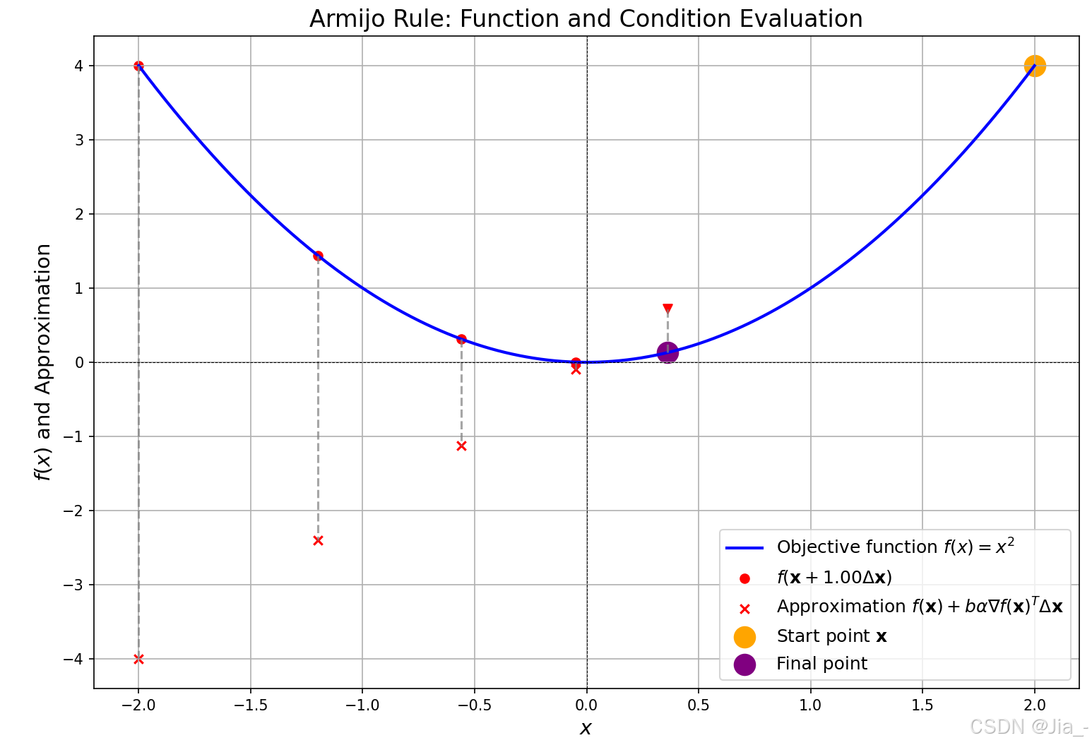
- b b b is tolerance, b ∈ ( 0 , 1 ) b \in (0,1) b∈(0,1).
- b α ∇ f ( x ) T Δ x b \alpha \nabla f(\mathbf{x})^T \Delta \mathbf{x} bα∇f(x)TΔx is the expected reduction from the gradient.
(2) Intuition
- Ensure the step agrees with linearization within some tolerance b b b.
- Typical values: b = 1 0 − 4 − 1 0 − 1 , c = 1 / 2 b = 10^{-4} - 10^{-1}, c = 1/2 b=10−4−10−1,c=1/2.
(3) Example: Backtracking Regularized Newton Step
function backtracking_regularized_newton_step(x0)
    b = 0.1
    c = 0.5
    β = 1.0
    H = ∇²f(x0)
    while !isposdef(H)
        H = H + β * I
    end
    Δx = -H \ ∇f(x0)

    α = 1.0
    while f(x0 + α * Δx) > f(x0) + b * α * ∇f(x0)' * Δx
        α = c * α
    end

    xn = x0 + α * Δx
end
(4) Takeaway Message
Newton’s method, with simple and cheap modifications (globalization strategy), is extremely effective at finding local minima.
2. Equality Constraints
Given
f
(
x
)
:
R
n
→
R
f(\mathbf{x}): \mathbb{R}^n \rightarrow \mathbb{R}
f(x):Rn→R ,
c
(
x
)
:
R
n
→
R
m
\mathbf{c}(\mathbf{x}): \mathbb{R}^n \rightarrow \mathbb{R}^m
c(x):Rn→Rm.
Problem:
min
x
f
(
x
)
s.t.
c
(
x
)
=
0
\min_{\mathbf{x}} f(\mathbf{x}) \\ \text{s.t.} \quad \mathbf{c}(\mathbf{x}) = \mathbf{0}
xminf(x)s.t.c(x)=0
(1) First-Order Necessary Conditions:
- ∇ f ( x ) = 0 \nabla f(\mathbf{x}) = 0 ∇f(x)=0 in free directions.
- c ( x ) = 0 \mathbf{c}(\mathbf{x}) = 0 c(x)=0.
Explanation:
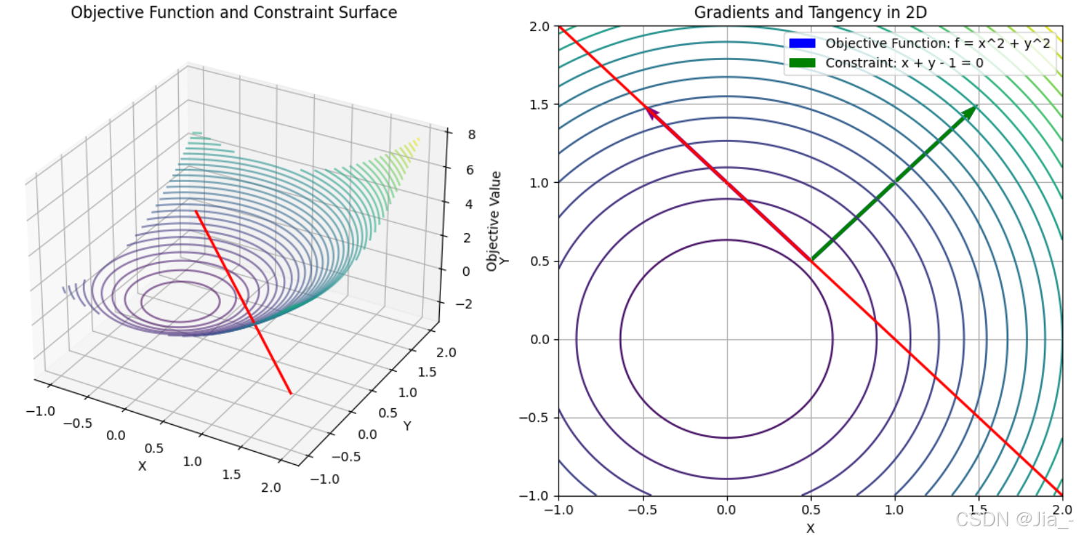
- If any component of ∇ f ( x ) \nabla f(\mathbf{x}) ∇f(x) is not normal to the constraint surface, we can reduce f ( x ) f(\mathbf{x}) f(x) by moving along the surface.
(2) Lagrange Multiplier
∇ f ( x ) + λ ∇ c ( x ) = 0 , λ ∈ R m \nabla f(\mathbf{x}) + \lambda \nabla \mathbf{c}(\mathbf{x}) = \mathbf{0}, \quad \lambda \in \mathbb{R}^m ∇f(x)+λ∇c(x)=0,λ∈Rm
- ∇ f ( x ) \nabla f(\mathbf{x}) ∇f(x) and ∇ c ( x ) \nabla \mathbf{c}(\mathbf{x}) ∇c(x) are parallel.
(3) Lagrangian
L ( x , λ ) = f ( x ) + λ ⊤ c ( x ) . L(\mathbf{x}, \lambda) = f(\mathbf{x}) + \lambda^\top \mathbf{c}(\mathbf{x}). L(x,λ)=f(x)+λ⊤c(x).
- Turns constrained minimization into an unconstrained problem:
min x L ( x , λ ) . \min_{\mathbf{x}}L(\mathbf{x}, \lambda). xminL(x,λ).
Gradients (KKT conditions):
∇ x L ( x , λ ) = ∇ f ( x ) + ( ∂ c ∂ x ) ⊤ λ = 0 , \nabla_xL(\mathbf{x}, \lambda) = \nabla f(\mathbf{x}) + \left(\frac{\partial \mathbf{c}}{\partial \mathbf{x}}\right)^\top \lambda = \mathbf{0}, ∇xL(x,λ)=∇f(x)+(∂x∂c)⊤λ=0, ∇ λ L ( x , λ ) = c ( x ) = 0. \nabla_\lambda L(\mathbf{x}, \lambda) = \mathbf{c}(\mathbf{x}) = \mathbf{0}. ∇λL(x,λ)=c(x)=0.
To solve equations where the gradient is zero, we employ Newton’s method. With two variables and two outputs (not necessarily two-dimensional), we perform a first-order Taylor expansion of the equation and set it to zero (since we are solving for roots). This yields an iterative formula for the roots of the equation, specifically for the local extrema of the Lagrangian function ( L(x, \lambda) ), analogous to Newton’s method for single-variable equations.
∇
x
L
(
x
+
Δ
x
,
λ
+
Δ
λ
)
≈
∇
x
L
(
x
,
λ
)
+
∂
2
L
∂
x
2
Δ
x
+
∂
2
L
∂
x
∂
λ
Δ
λ
=
0
\nabla_x L(x + \Delta x, \lambda + \Delta \lambda) \approx \nabla_x L(x, \lambda) + \frac{\partial^2 L}{\partial x^2} \Delta x + \frac{\partial^2 L}{\partial x \partial \lambda} \Delta \lambda = 0
∇xL(x+Δx,λ+Δλ)≈∇xL(x,λ)+∂x2∂2LΔx+∂x∂λ∂2LΔλ=0Where:
∂
2
L
∂
x
∂
λ
=
∂
2
L
∂
λ
∂
x
=
∂
∂
x
(
∂
L
∂
λ
)
=
(
∂
C
∂
x
)
T
\frac{\partial^2 L}{\partial x \partial \lambda} = \frac{\partial^2 L}{\partial \lambda \partial x} = \frac{\partial}{\partial x} \left( \frac{\partial L}{\partial \lambda} \right) = \left( \frac{\partial C}{\partial x} \right)^T
∂x∂λ∂2L=∂λ∂x∂2L=∂x∂(∂λ∂L)=(∂x∂C)T
For ∇ λ L \nabla_\lambda L ∇λL:
∇ λ L ( x + Δ x , λ + Δ λ ) = C ( x ) + ∂ C ∂ x Δ x = 0 ⇒ ∂ C ∂ x Δ x = − C ( x ) \nabla_{\lambda} L(x + \Delta x, \lambda + \Delta \lambda) = C(x) + \frac{\partial C}{\partial x} \Delta x = 0 \Rightarrow \frac{\partial C}{\partial x} \Delta x = -C(x) ∇λL(x+Δx,λ+Δλ)=C(x)+∂x∂CΔx=0⇒∂x∂CΔx=−C(x)
Explanation of Symbols
-
L ( x , λ ) L(x, \lambda) L(x,λ): The Lagrangian function, typically the combination of the objective function and constraints.
L ( x , λ ) = f ( x ) + λ T C ( x ) L(x, \lambda) = f(x) + \lambda^T C(x) L(x,λ)=f(x)+λTC(x)Here, λ \lambda λrepresents the Lagrange multipliers. -
∇ x L ( x , λ ) \nabla_x L(x, \lambda) ∇xL(x,λ): The gradient of L ( x , λ ) L(x, \lambda) L(x,λ) with respect to x x x, representing the rate of change of the objective function along the directions of x x x.
-
∇ x L ( x + α Δ x , λ + Δ λ ) \nabla_x L(x + \alpha \Delta x, \lambda + \Delta \lambda) ∇xL(x+αΔx,λ+Δλ): The gradient of L L L at the updated point ( x + α Δ x , λ + Δ λ ) (x + \alpha \Delta x, \lambda + \Delta \lambda) (x+αΔx,λ+Δλ), where α \alpha α is the step size, and Δ x , Δ λ \Delta x, \Delta \lambda Δx,Δλ are the increments of x x x and λ \lambda λ, respectively.
-
∂ 2 L ∂ x 2 \frac{\partial^2 L}{\partial x^2} ∂x2∂2L: The second derivative of L L L with respect to x x x, indicating the curvature of the objective function along x x x.
-
∂ 2 L ∂ x ∂ λ \frac{\partial^2 L}{\partial x \partial \lambda} ∂x∂λ∂2L: The mixed second derivative of L L L with respect to x x x and λ \lambda λ, representing interactions between the variables.
-
Δ x , Δ λ \Delta x, \Delta \lambda Δx,Δλ: The updates for the optimization variables x x x and the Lagrange multipliers λ \lambda λ.
Derivation 1: ∇ x L ( x + Δ x , λ + Δ λ ) \nabla_x L(x + \Delta x, \lambda + \Delta \lambda) ∇xL(x+Δx,λ+Δλ)
1. Taylor Expansion
Using the first-order Taylor expansion for L ( x , λ ) L(x, \lambda) L(x,λ), where x x x and λ \lambda λ undergo small changes Δ x \Delta x Δx and Δ λ \Delta \lambda Δλ, we have:
L ( x + Δ x , λ + Δ λ ) ≈ L ( x , λ ) + ∇ x L ( x , λ ) ⋅ Δ x + ∇ λ L ( x , λ ) ⋅ Δ λ L(x + \Delta x, \lambda + \Delta \lambda) \approx L(x, \lambda) + \nabla_x L(x, \lambda) \cdot \Delta x + \nabla_\lambda L(x, \lambda) \cdot \Delta \lambda L(x+Δx,λ+Δλ)≈L(x,λ)+∇xL(x,λ)⋅Δx+∇λL(x,λ)⋅ΔλFor the gradient with respect to x x x, we expand ∇ x L ( x + Δ x , λ + Δ λ ) \nabla_x L(x + \Delta x, \lambda + \Delta \lambda) ∇xL(x+Δx,λ+Δλ) as follows:
∇ x L ( x + Δ x , λ + Δ λ ) ≈ ∇ x L ( x , λ ) + ∂ 2 L ∂ x 2 Δ x + ∂ 2 L ∂ x ∂ λ Δ λ \nabla_x L(x + \Delta x, \lambda + \Delta \lambda) \approx \nabla_x L(x, \lambda) + \frac{\partial^2 L}{\partial x^2} \Delta x + \frac{\partial^2 L}{\partial x \partial \lambda} \Delta \lambda ∇xL(x+Δx,λ+Δλ)≈∇xL(x,λ)+∂x2∂2LΔx+∂x∂λ∂2LΔλHere:
∂ 2 L ∂ x 2 Δ x \frac{\partial^2 L}{\partial x^2} \Delta x ∂x2∂2LΔx: The contribution from the second-order derivative with respect to x x x, describing how the gradient changes due to x x x.
∂ 2 L ∂ x ∂ λ Δ λ \frac{\partial^2 L}{\partial x \partial \lambda} \Delta \lambda ∂x∂λ∂2LΔλ: The contribution from the mixed second-order derivative with respect to x x x and λ \lambda λ, describing the interaction between the two variables.
Setting this equation to zero (since we are solving for the critical points of the gradient):
∇ x L ( x + Δ x , λ + Δ λ ) = 0 ⇒ ∇ x L ( x , λ ) + ∂ 2 L ∂ x 2 Δ x + ∂ 2 L ∂ x ∂ λ Δ λ = 0 \nabla_x L(x + \Delta x, \lambda + \Delta \lambda) = 0 \Rightarrow \nabla_x L(x, \lambda) + \frac{\partial^2 L}{\partial x^2} \Delta x + \frac{\partial^2 L}{\partial x \partial \lambda} \Delta \lambda = 0 ∇xL(x+Δx,λ+Δλ)=0⇒∇xL(x,λ)+∂x2∂2LΔx+∂x∂λ∂2LΔλ=0
Derivation 2: ∂ 2 L ∂ x ∂ λ \frac{\partial^2 L}{\partial x \partial \lambda} ∂x∂λ∂2L
Using the symmetry property of mixed second-order derivatives, we know:
∂ 2 L ∂ x ∂ λ = ∂ 2 L ∂ λ ∂ x \frac{\partial^2 L}{\partial x \partial \lambda} = \frac{\partial^2 L}{\partial \lambda \partial x} ∂x∂λ∂2L=∂λ∂x∂2LFrom the definition of the Lagrangian function:
L ( x , λ ) = f ( x ) + λ T C ( x ) L(x, \lambda) = f(x) + \lambda^T C(x) L(x,λ)=f(x)+λTC(x)where:
f ( x ) f(x) f(x): Objective function.
C ( x ) C(x) C(x): Constraint function.
The derivative of L L L with respect to λ \lambda λ is:
∂ L ∂ λ = C ( x ) \frac{\partial L}{\partial \lambda} = C(x) ∂λ∂L=C(x)Taking the derivative of ∂ L ∂ λ \frac{\partial L}{\partial \lambda} ∂λ∂L with respect to x x x:
∂ ∂ x ( ∂ L ∂ λ ) = ∂ ∂ x ( C ( x ) ) \frac{\partial}{\partial x} \left( \frac{\partial L}{\partial \lambda} \right) = \frac{\partial}{\partial x} \left( C(x) \right) ∂x∂(∂λ∂L)=∂x∂(C(x))Thus: ∂ 2 L ∂ x ∂ λ = ( ∂ C ∂ x ) T \frac{\partial^2 L}{\partial x \partial \lambda} = \left( \frac{\partial C}{\partial x} \right)^T ∂x∂λ∂2L=(∂x∂C)T
Derivation 3: ∇ λ L ( x + Δ x , λ + Δ λ ) \nabla_\lambda L(x + \Delta x, \lambda + \Delta \lambda) ∇λL(x+Δx,λ+Δλ)
From the definition of the Lagrangian:
L ( x , λ ) = f ( x ) + λ T C ( x ) L(x, \lambda) = f(x) + \lambda^T C(x) L(x,λ)=f(x)+λTC(x)The gradient with respect to λ \lambda λ is:
∇ λ L ( x , λ ) = C ( x ) \nabla_\lambda L(x, \lambda) = C(x) ∇λL(x,λ)=C(x)Expanding ∇ λ L \nabla_\lambda L ∇λL using the first-order Taylor expansion:
∇ λ L ( x + Δ x , λ + Δ λ ) ≈ ∇ λ L ( x , λ ) + ∂ ∂ λ ( ∇ λ L ( x , λ ) ) Δ λ + ∂ ∂ x ( ∇ λ L ( x , λ ) ) Δ x \nabla_\lambda L(x + \Delta x, \lambda + \Delta \lambda) \approx \nabla_\lambda L(x, \lambda) + \frac{\partial}{\partial \lambda} \left( \nabla_\lambda L(x, \lambda) \right) \Delta \lambda + \frac{\partial}{\partial x} \left( \nabla_\lambda L(x, \lambda) \right) \Delta x ∇λL(x+Δx,λ+Δλ)≈∇λL(x,λ)+∂λ∂(∇λL(x,λ))Δλ+∂x∂(∇λL(x,λ))ΔxSince C ( x ) C(x) C(x) depends only on x x x and not on λ \lambda λ, we have ∂ C ( x ) ∂ λ = 0 \frac{\partial C(x)}{\partial \lambda} = 0 ∂λ∂C(x)=0. Therefore:
∇ λ L ( x + Δ x , λ + Δ λ ) ≈ C ( x ) + ∂ C ∂ x Δ x \nabla_\lambda L(x + \Delta x, \lambda + \Delta \lambda) \approx C(x) + \frac{\partial C}{\partial x} \Delta x ∇λL(x+Δx,λ+Δλ)≈C(x)+∂x∂CΔxSetting this equation to zero:
C ( x ) + ∂ C ∂ x Δ x = 0 ⇒ ∂ C ∂ x Δ x = − C ( x ) C(x) + \frac{\partial C}{\partial x} \Delta x = 0 \Rightarrow \frac{\partial C}{\partial x} \Delta x = -C(x) C(x)+∂x∂CΔx=0⇒∂x∂CΔx=−C(x)
Iterative Formula and the KKT System
Combining the above, we derive the iterative formula for ( x ) and ( \lambda ):
[
∂
2
L
∂
x
2
(
∂
C
∂
x
)
T
∂
C
∂
x
0
]
[
Δ
x
Δ
λ
]
=
[
−
∇
x
L
(
x
,
λ
)
−
C
(
x
)
]
\begin{bmatrix} \frac{\partial^2 L}{\partial x^2} & \left(\frac{\partial C}{\partial x}\right)^T \\ \frac{\partial C}{\partial x} & 0 \end{bmatrix} \begin{bmatrix} \Delta x \\ \Delta \lambda \end{bmatrix} =\begin{bmatrix} -\nabla_x L(x, \lambda) \\ -C(x) \end{bmatrix}
[∂x2∂2L∂x∂C(∂x∂C)T0][ΔxΔλ]=[−∇xL(x,λ)−C(x)]
This matrix system is referred to as the KKT system (Karush-Kuhn-Tucker system). The top-left block represents the Hessian matrix of the Lagrangian function.
Special Solvers for the KKT System
Due to the specific structure and generality of this matrix, there are many targeted solvers designed to efficiently iterate through and solve the KKT system, as noted in lectures.
3. Gauss-Newton Method
(1) Basic Idea
In the KKT system, there is a term involving the second derivative of L L L with respect to x x x, which includes the second derivative of the objective function and the curvature term of the constraint. In practical problems, f f f is the desired objective function, which can be designed to be relatively well-behaved, while c c c represents the constraints, which come from real physical systems and are often more complex and difficult to differentiate. Therefore, when iterating over the KKT system, it is possible to consider discarding the second term of the second derivative of L L L, i.e., ∂ 2 L ∂ x 2 \frac{\partial^2 L}{\partial x^2} ∂x2∂2L. This method is known as the Gauss-Newton method. The Gauss-Newton method is equivalent to first linearizing the system and then solving for the extremum points of the linearized system.
∂ 2 L ∂ x 2 = ∇ 2 f ( x ) + ∂ ∂ x [ ( ∂ c ∂ x ) ⊤ λ ] ≈ ∇ 2 f ( x ) . \frac{\partial^2L}{\partial \mathbf{x}^2} = \nabla^2 f(\mathbf{x}) + \frac{\partial}{\partial \mathbf{x}}\left[\left(\frac{\partial \mathbf{c}}{\partial \mathbf{x}}\right)^\top \lambda\right] \approx \nabla^2 f(\mathbf{x}). ∂x2∂2L=∇2f(x)+∂x∂[(∂x∂c)⊤λ]≈∇2f(x).
- The second term is expensive to compute, so it is dropped.
- Gauss-Newton method has slower convergence than Newton’s method but is computationally cheaper per iteration.
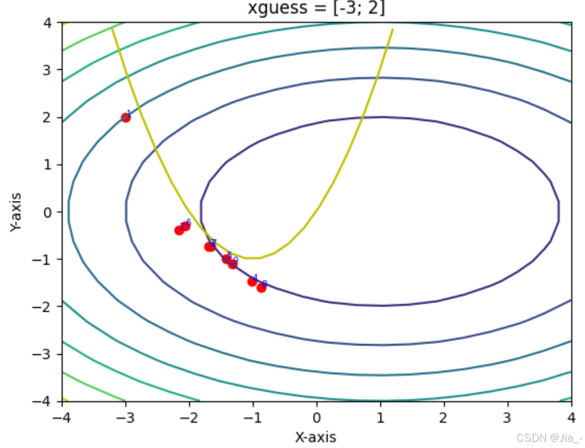
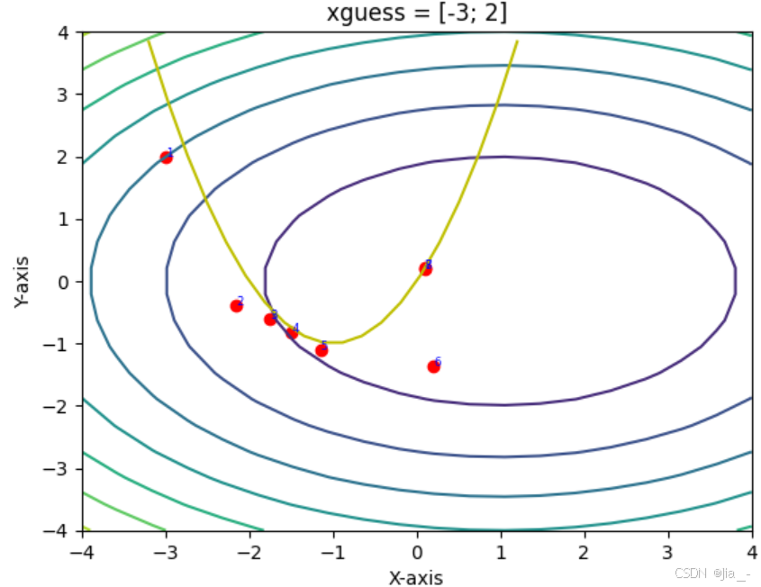
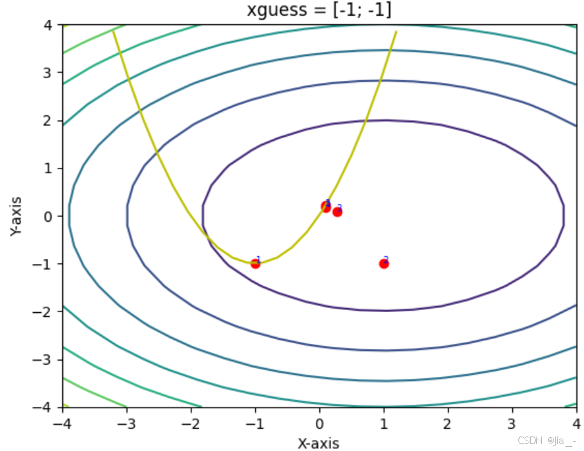
(2) Example: Comparison of Newton vs. Gauss-Newton1
Using Newton’s method and Gauss-Newton’s method, the problem depicted in the figure below is minimized. The concentric circles represent the contour lines of the objective function, while the yellow parabola indicates the constraint. It can be observed that Newton’s method, starting from an unreasonable initial point (-3, 2), may fail to converge to the local minimum. In contrast, the Gauss-Newton method does not encounter this issue. By removing the second term, the Gauss-Newton method ensures that the Hessian matrix is positive definite, guaranteeing that each iteration moves in a descending direction. Although Newton’s method theoretically converges faster near the vicinity of the extremum, in practice, the Gauss-Newton method demonstrates greater stability.
-
Newton’s Method: Typically fewer iterations but higher cost per iteration.

-
Gauss-Newton Method: Cheaper per iteration but slower convergence.
(3) Takeaway Message
May still need to regularize the Hessian:
∂ 2 L ∂ x 2 \frac{\partial^2 L}{\partial \mathbf{x}^2} ∂x2∂2L
even if:
∇ 2 f ( x ) ≻ 0 \nabla^2 f\left(\mathbf{x}\right) \succ 0 ∇2f(x)≻0
The Gauss-Newton method is often used in practice.
(4) Inequality Constraints
Minimize f ( x ) f(x) f(x) subject to c ( x ) ≤ 0 c(x) \leq 0 c(x)≤0:
min x f ( x ) s.t. c ( x ) ≤ 0 \min_{\mathbf{x}} f\left(\mathbf{x}\right) \quad \text{s.t.} \quad \mathbf{c}\left(\mathbf{x}\right) \leq \mathbf{0} xminf(x)s.t.c(x)≤0We’ll look at just inequality constraints for now. These are handled by combining with previous methods for both types of constraints.
First-Order Necessary Conditions
i. Need:
∇ f ( x ) = 0 \nabla f\left(\mathbf{x}\right) = \mathbf{0} ∇f(x)=0 in free directions.
ii. Need:
c
(
x
)
≤
0
\mathbf{c}\left(\mathbf{x}\right) \leq \mathbf{0}
c(x)≤0(Same as equality constraints)
(i) KKT Conditions
The Karush-Kuhn-Tucker (KKT) conditions are:
∇ f ( x ) + ( ∂ c ∂ x ) ⊤ λ = 0 ( stationarity ) \nabla f(\mathbf{x}) + \left( \frac{\partial c}{\partial x} \right)^\top \lambda = 0 \quad (\text{stationarity}) ∇f(x)+(∂x∂c)⊤λ=0(stationarity)
c ( x ) ≤ 0 ( primal feasibility ) c(\mathbf{x}) \leq 0 \quad (\text{primal feasibility}) c(x)≤0(primal feasibility)
λ ≥ 0 ( dual feasibility ) \lambda \geq 0 \quad (\text{dual feasibility}) λ≥0(dual feasibility)
λ ⊙ c ( x ) = λ ⊤ c ( x ) = 0 ( complementary slackness ) \lambda \odot c(\mathbf{x}) = \lambda^\top c(\mathbf{x}) = 0 \quad (\text{complementary slackness}) λ⊙c(x)=λ⊤c(x)=0(complementary slackness) for some λ ∈ R m \lambda \in \mathbb{R}^m λ∈Rm.
(ii) Intuition of KKT Conditions
- If the constraint is active ( c ( x ) = 0 c(\mathbf{x}) = 0 c(x)=0), then λ > 0 \lambda > 0 λ>0.
- If the constraint is inactive ( c ( x ) < 0 c(\mathbf{x}) < 0 c(x)<0), then λ = 0 \lambda = 0 λ=0.
(iii) Takeaway Message
The complementary slackness condition is like a switch:
- If the constraint is active, the switch is on ( λ > 0 \lambda > 0 λ>0).
- If the constraint is inactive, the switch is off ( λ = 0 \lambda = 0 λ=0).
Additionally, there is an edge case when the minimum of the objective happens to be on the constraint manifold, i.e., when c ( x ) = λ = 0 c(\mathbf{x}) = \lambda = 0 c(x)=λ=0.
From KKT Condition, it can be seen that the first-order necessary conditions for inequality constraints are mathematically complex. Moreover, the complementary slackness condition introduces powerful nonlinearity, even an if-else logic, which makes finding the minimum point from KKT Condition relatively complicated. Therefore, alternative methods must be sought. Additionally, the KKT conditions only tell us what the situation looks like at the extremum points but do not provide a method for iteration or optimization to reach the extremum points. Hence, how to solve this problem and how to handle the different cases depends on the specific solver being used.
References
[1] 【2024 Optimal Control and Reinforcement Learning 16-745】【Lecture 4】优化(中)——线搜索(Armijo准则)、约束最小化
[2] 【Optimal Control (CMU 16-745)】Lecture 3 Optimization Part 2
[3] Lecture 4 约束最优化问题
[4] CMU Optimal Control 16-745 Video From Bilibili
[5] CMU Optimal Control 16-745
感谢大家阅读这篇学习笔记!记录学习的内容,如果有问题或者不准确的地方,欢迎随时联系我改正,与大家共同进步!


 被折叠的 条评论
为什么被折叠?
被折叠的 条评论
为什么被折叠?
 到【灌水乐园】发言


