


'''自主构建数据集'''
import matplotlib.pyplot as plt
import numpy as np
from matplotlib.colors import ListedColormap
from sklearn.model_selection import train_test_split
from sklearn.datasets import make_moons
from sklearn.svm import SVC
X, y = make_moons(n_samples=500, noise=0.30, random_state=42)
X_train, X_test, y_train, y_test = train_test_split(X, y, random_state=42)
m = len(X_train)
def plot_decision_boundary(clf, X, y, axes=[-1.5, 2.5, -1, 1.5], alpha=0.5, contour=True):
'''
:param clf: 传入的模型
:param X: 用于分析的原始数据X
:param y: 原始数据y
:param axes: 坐标范围 前两个为X范围 后两个为y范围
:param alpha: 透明度
:param contour: 是否绘制等高线
:return:
'''
'''绘制坐标棋盘'''
x1s = np.linspace(axes[0], axes[1], 100)
x2s = np.linspace(axes[2], axes[3], 100)
# 构建棋盘
x1, x2 = np.meshgrid(x1s, x2s)
##在棋盘中构建待测试数据
X_new = np.c_[x1.ravel(), x2.ravel()]
##预测最终结果值
y_pred = clf.predict(X_new).reshape(x1.shape)
custom_cmap = ListedColormap(['#fafab0', '#9898ff', '#a0faa0'])
plt.contourf(x1, x2, y_pred, cmap=custom_cmap, alpha=0.3) ##进行填充
'''绘制等高线'''
if contour:
custom_cmap2 = ListedColormap(['#7d7d58', '#4c4c7f', '#507d50'])
plt.contour(x1, x2, y_pred, cmap=custom_cmap2, alpha=0.8)
'''绘制数据点'''
plt.plot(X[:, 0][y == 0], X[:, 1][y == 0], 'yo', alpha=0.6)
plt.plot(X[:, 0][y == 1], X[:, 1][y == 1], 'bs', alpha=0.6)
plt.axis(axes)
plt.xlabel('x1')
plt.xlabel('x2')
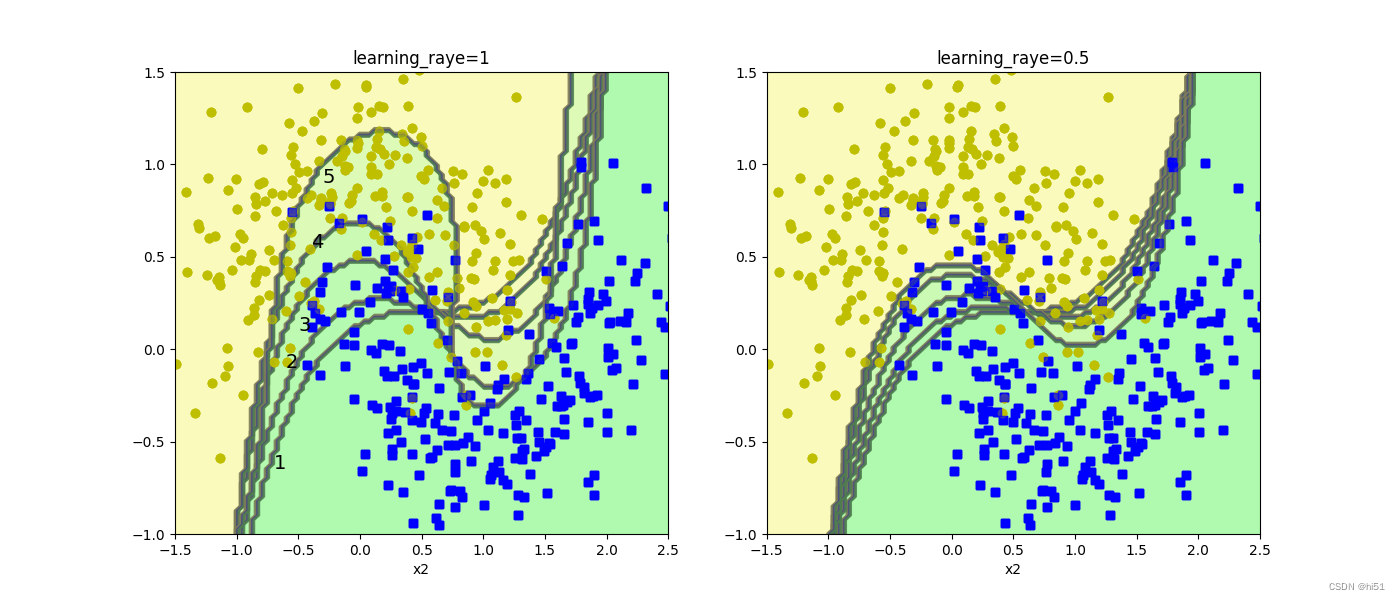
'''绘图展示随着集成算法的进行 决策边界的改变'''
###不同的调节力度对结果的影响 学习率(样本权重更新的速度)
plt.figure(figsize=(14, 5))
for subplot, learing_rate in ((121, 1), (122, 0.5)):
sample_weights = np.ones(m) ##最开始每个样本的权重是相同的
plt.subplot(subplot) ##将当前子图编号传入
####对模型与样本的权重进行更新
for i in range(5):
svm_clf = SVC(kernel="rbf", C=0.05, random_state=42)
###kernel:核函数 此处使用高斯核函数 C:软间隔
svm_clf.fit(X_train, y_train, sample_weight=sample_weights) ##训练过程不仅可以指定XY 还可以指定样本的权重项
y_pred = svm_clf.predict(X_train) ##训练集通过模型得到的结果
'''调节权重参数 将判断错误的参数更改
此处权重参数的改变并没有使用论文中的公式 而是使用学习率进行简单更改'''
sample_weights[y_pred != y_train] *= (1 + learing_rate)
###每次执行完毕后绘制决策边界
plot_decision_boundary(svm_clf, X, y, alpha=0.2)
plt.title("learning_raye={}".format(learing_rate))
if subplot == 121:
plt.text(-0.7, -0.65, "1", fontsize=14)
plt.text(-0.6, -0.10, "2", fontsize=14)
plt.text(-0.5, 0.10, "3", fontsize=14)
plt.text(-0.4, 0.55, "4", fontsize=14)
plt.text(-0.3, 0.90, "5", fontsize=14)
plt.show()上述代码运行效果如下:
Sklearn中关于AdaBoost算法的API文档:sklearn.ensemble.AdaBoostClassifier-scikit-learn中文社区
运行实例如下:
'''使用sklearn工具包实现AdaBoost算法'''
from sklearn.ensemble import AdaBoostClassifier
from sklearn.tree import DecisionTreeClassifier

ada_clf = AdaBoostClassifier(
    base_estimator=DecisionTreeClassifier(max_depth=1),  ##传入的树模型 此处为了展示效果好将深度设置为1
    n_estimators=200,  ##模型运行的轮次
    learning_rate=0.5,  ##学习率
    random_state=42
)
ada_clf.fit(X_train, y_train)
##绘制决策边界
plot_decision_boundary(ada_clf, X, y, alpha=0.2)
plt.show()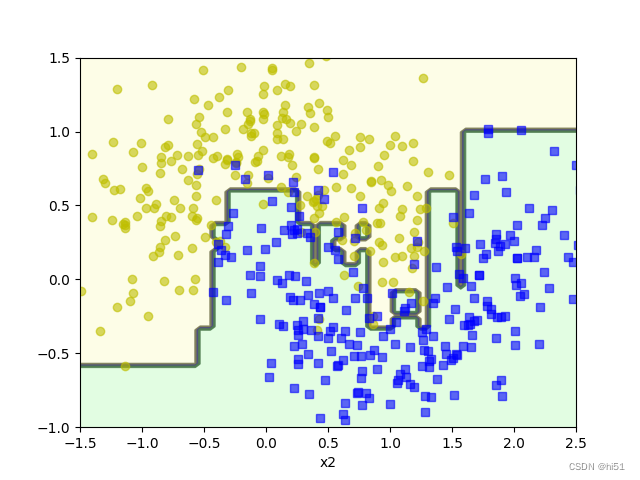


 652
652


 被折叠的 条评论
为什么被折叠?
被折叠的 条评论
为什么被折叠?
 到【灌水乐园】发言


