


RNN
什么是循环神经网路
Recurrent Neural Networ(RNN),是一类具有内部环状连接的人工神经网络。用于处理序列数据。
简单代码示例
# 一个简单的RNN结构示例
class SimpleRNN(nn.Module):
    def __init__(self, input_size, hidden_size):
        super(SimpleRNN, self).__init__()
        self.rnn = nn.RNN(input_size, hidden_size, batch_first=True)

    def forward(self, x):
        out, _ = self.rnn(x)
        return out
网络结构
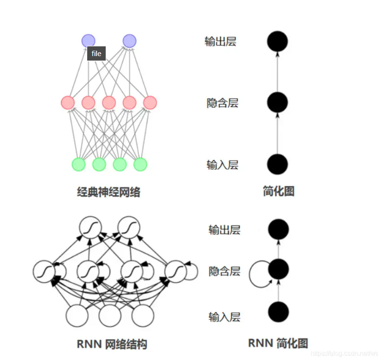
基础结构
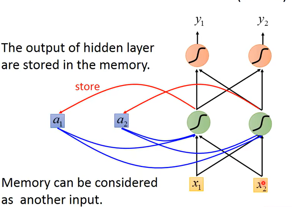
有点像全连接层,但是在全连接层的基础上,将隐藏层最后的值多考虑了上一次隐藏层的值。也就是得到的最后的输出值,即考虑了现在的输入也考虑了以前的输入。具有记忆功能。
上图假设输入的第一个序列有两个维度分别为x1, x2, 中间有个隐藏层(hiddenl layer)有着记忆功能,最后隐藏层输出预测值。
Example
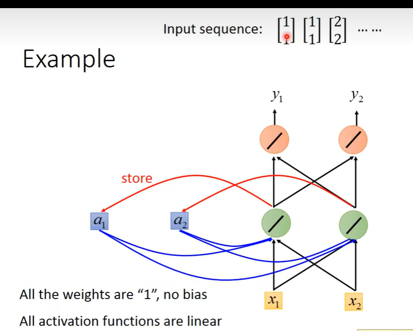
假设输入一连串序列,所有的权重都为1,没有bias。所有的激活函数都为f(x) = x。隐藏层初始化为[0,0]
-
先输入第一个序列[1,1],
a1 = a1*1 + a2*1+x1*1+x2*1
= 0 + 0 + 1 + 1 = 2a2 = a1 + a2 + x1 + x2
= 0 + 0 + 1 + 1 = 2y1 = a1 + a2 = 4
y2 = a1 + a2 = 4 -
输入第二个序列 [1, 1]
a1 = a1 + a2 + x1 + x2
= 2 + 2 + 1 + 1
= 6
a2 = a1 + a2 + x1 + x2
= 2 + 2 + 1 + 1
= 6y1 = a1 + a2 = 12
y2 = a1 + a2 = 12
-
输入第三个序列 [2, 2]
a1 = a1 + a2 + x1 + x2
= 6+ 6 + 2 + 2
= 16a2 = a1 + a2 + x1 + x2
= 6+ 6 + 2 + 2
= 16
y1 = a1 + a2 = 32y2 = a1 + a2 = 32
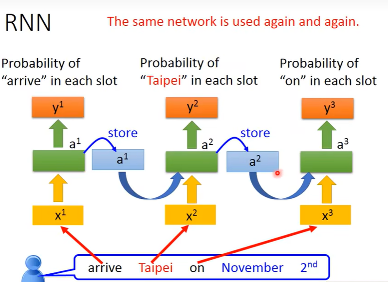
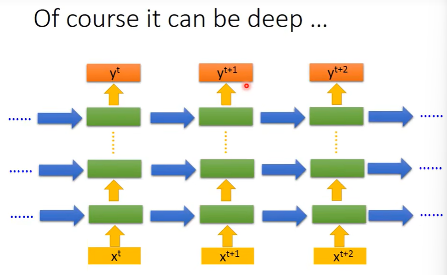
实际例子的直观运算过程,需要注意的是,每一次序列的运算用的都是同一组参数。(下图同种颜色的箭头用的参数代表同一组参数)
当然这个隐藏层可以是多层组成的
不同变形
Elman Network(前面讲的)
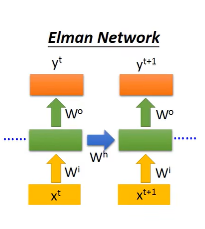
上一次hidden layer的输出作为这次hidden layer的输入。
Jordan Network
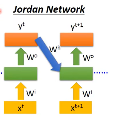
上一次的ouput的值作为下次hidden layer的输入。
Bidirectional RNN(双向RNN)
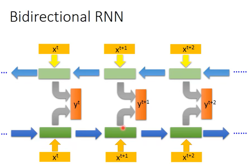
就是先运算正向RNN和反向RNN,最后结合正向和反向得到最后的输出值。分别考虑了序列的前面和后面(结合上下文)。
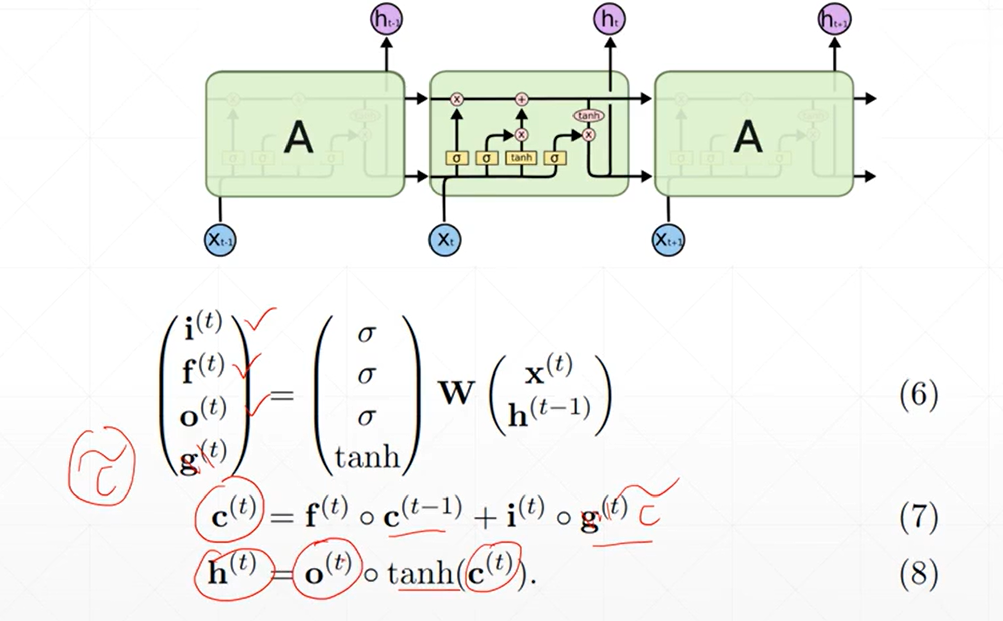
Long Short-term Memory(LSTM)
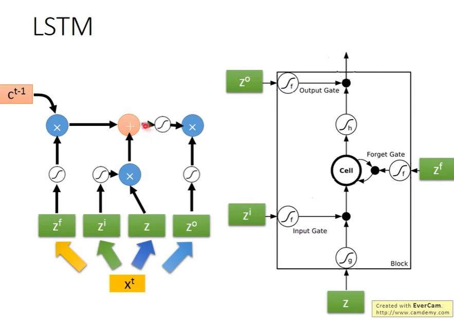
基本组成
有三个部分(3个阀门)组成:
- Input Gate
- Output Gate
- Forget Gate
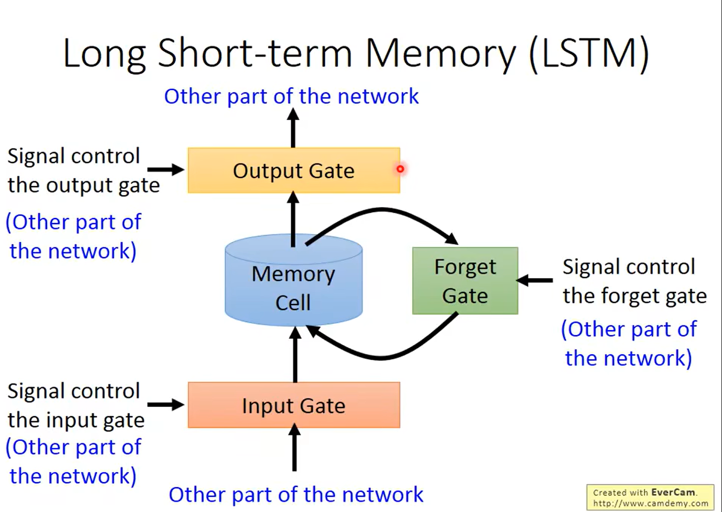
一共有4 Inputs, 1 Output
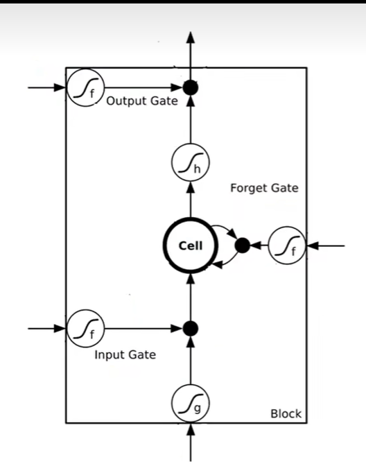
仔细来看,激活函数通常为sigmoid, 范围在0~1之间,代表阀门的打开程度。
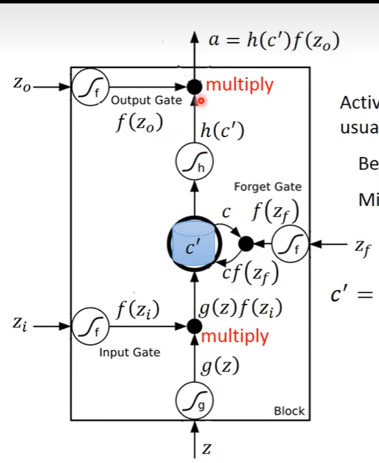
整个运算过程,
首先输入z->g(z), zi->f(zi), out1 = g(z)f(zi),
然后 zf->f(zf), c’=c*f(zf) + out1,
最后z0->f(z0), c’=h(c’), out = h(c’)f(z0)
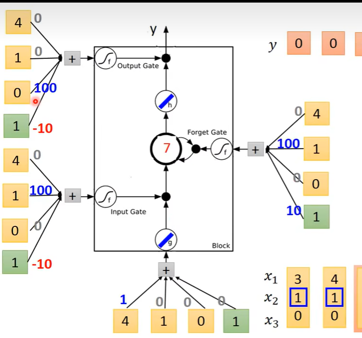
Example
四个Input的来源是序列的输入分别乘以四组不同的权重得来的。这些权重是可训练的。
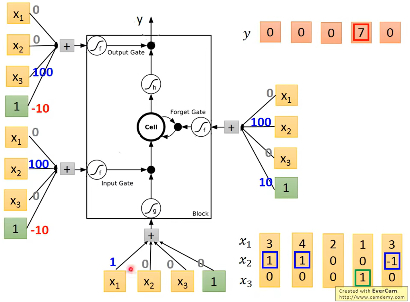
-
第一个序列输入
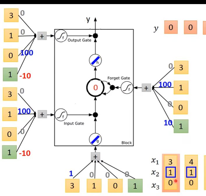
计算得到
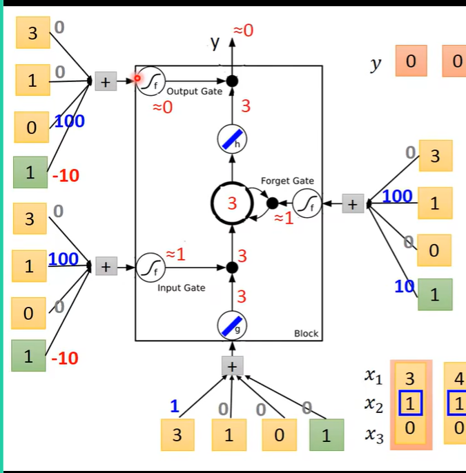
-
第二个序列输入
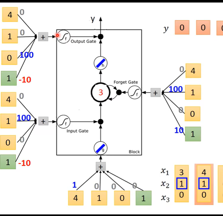
计算得到
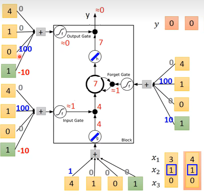
-
第三个序列输入
计算得到
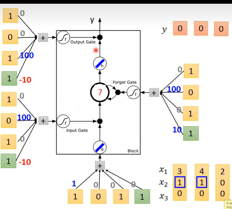
-
依次类推
完成LSTM组成
对比原来的RNN
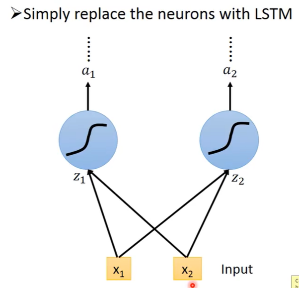
LSTM
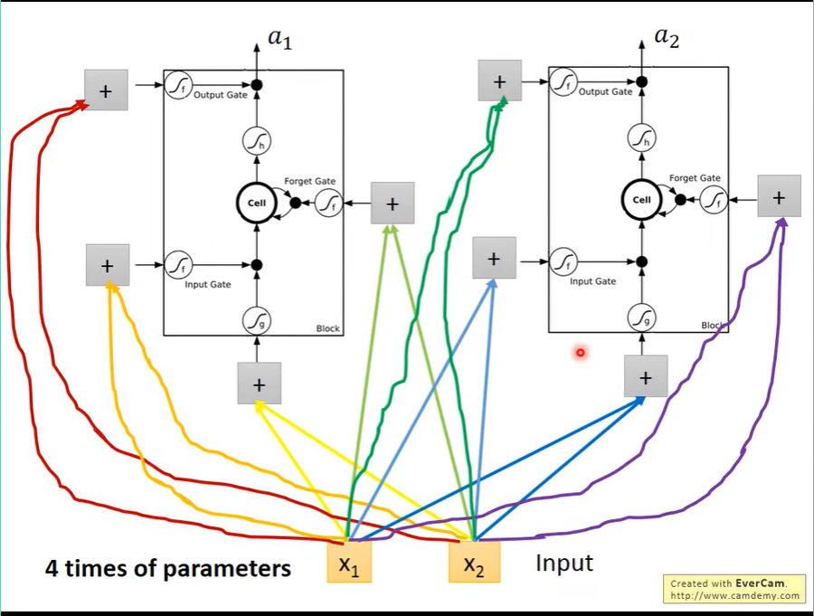
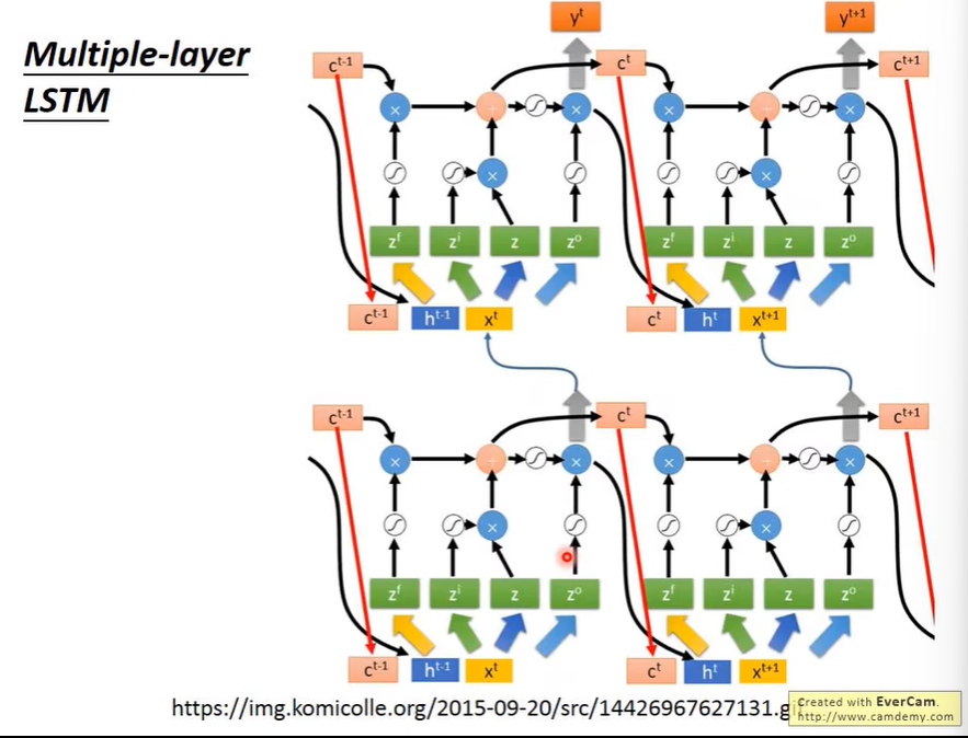
完整的LSTM
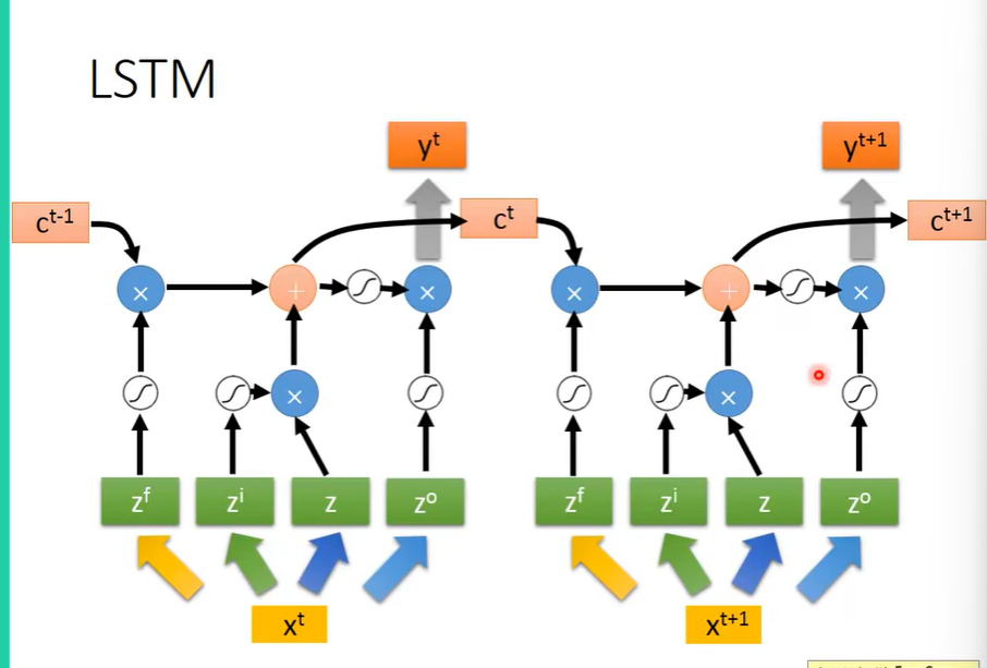
完整的LSTM会将上一次的输出作为这次的输入,
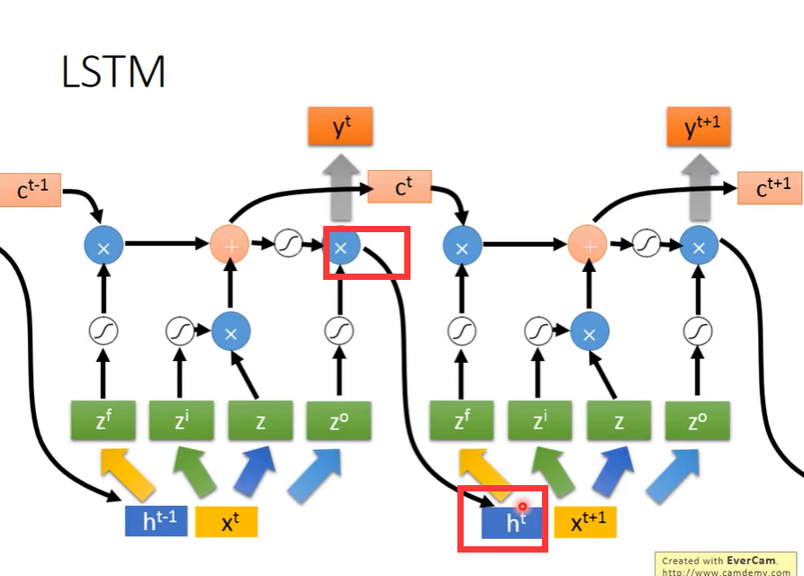
同时会将Cell里面的值作为这次的输入。
上图就是完整的LSTM形态。
Pytorch实现RNN
RNN代码讲解
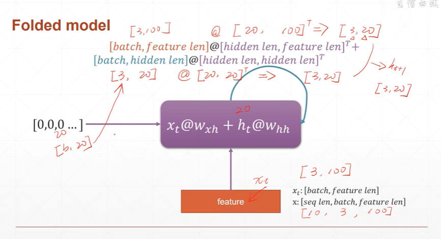
首先数据集x:[seq_len, batch, feature_len], xt:[batch, feature_len]
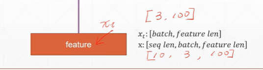
假设数据集x为10个序列,3个batch, 100维特征
每次的输入xt为3个batch,100维特征。
计算过程:
hidden_len=20
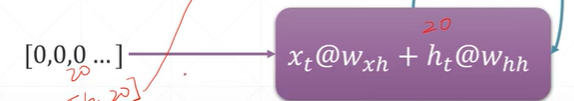
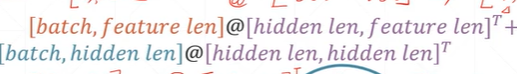
x(t)@w(xh) + h(t)@w(hh)
= [3, 100] @ [20, 100].T + [3, 20] @ [20, 20].T
=[3, 20] + [3,20]
= [3, 20]
Pytorch函数
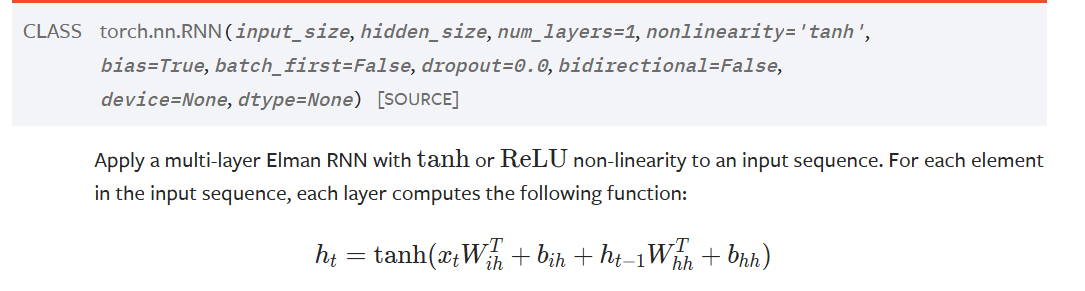
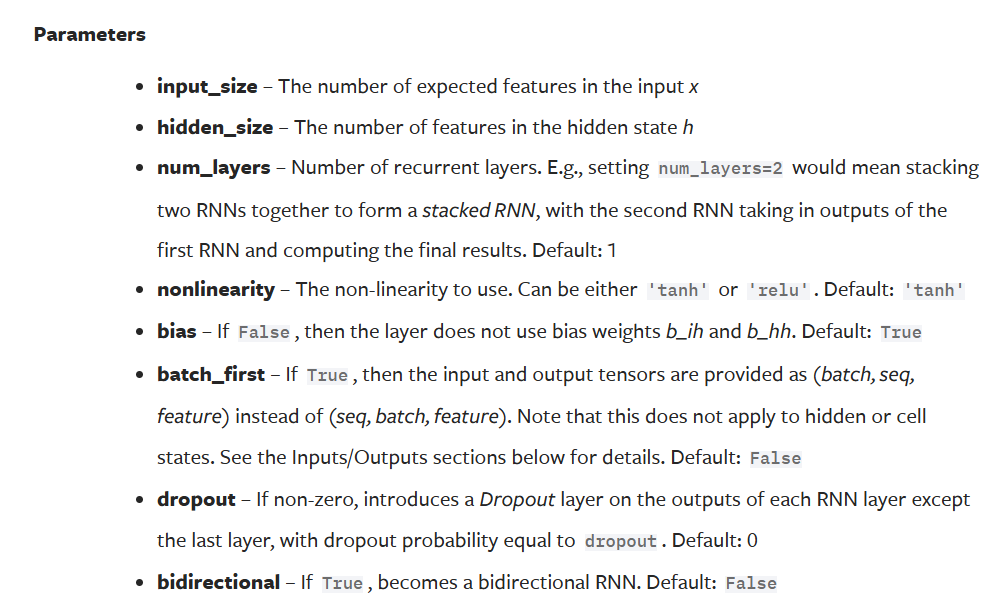
forward前向传播
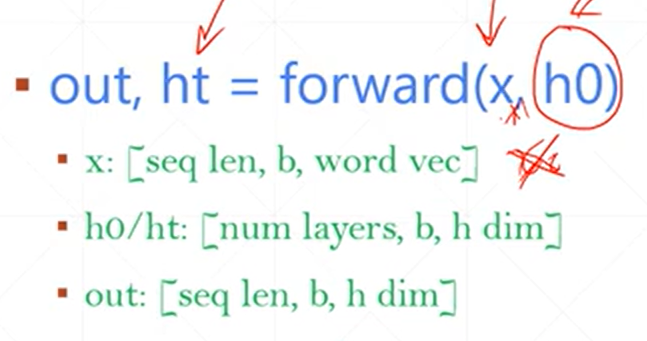
forward一步到位。
代码示例
import torch
from torch import nn
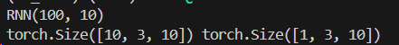
rnn = nn.RNN(input_size=100, hidden_size=10, num_layers=1)
print(rnn)
x = torch.randn(10, 3, 100) # 10 seq, 3 batch, 100 dim
out, h = rnn(x)
print(out.shape, h.shape)
运行结果
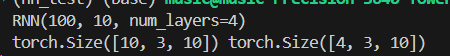
多层隐藏层代码
import torch
from torch import nn

rnn = nn.RNN(input_size=100, hidden_size=10, num_layers=4)
print(rnn)

x = torch.randn(10, 3, 100) # 10 seq, 3 batch, 100 dim
out, h = rnn(x)
print(out.shape, h.shape)
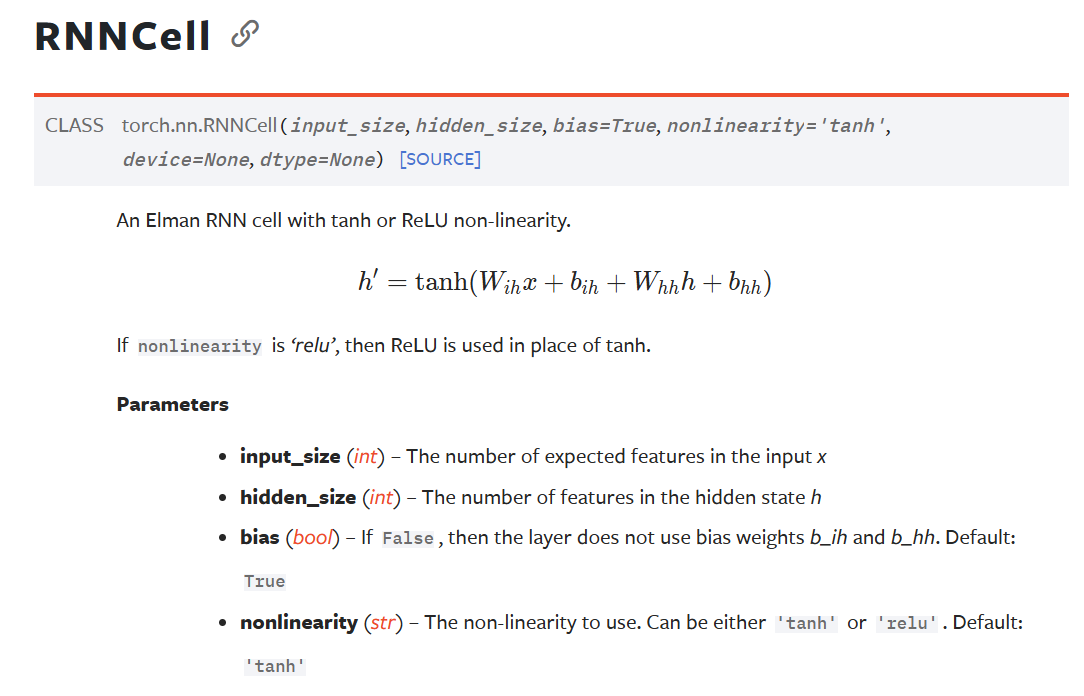
单次计算每次序列
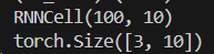
代码
import torch
from torch import nn
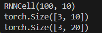
rnn = nn.RNNCell(input_size=100, hidden_size=10)
print(rnn)
x = torch.randn(10, 3, 100) # 10 seq, 3 batch, 100 dim
ht = torch.zeros(3, 10)
for xt in x:
ht = rnn(xt, ht)
print(ht.shape)
多层cell代码实现
import torch
from torch import nn

rnn1 = nn.RNNCell(input_size=100, hidden_size=10)
print(rnn1)
rnn2 = nn.RNNCell(input_size=10, hidden_size=20)

x = torch.randn(10, 3, 100) # 10 seq, 3 batch, 100 dim
ht1 = torch.zeros(3, 10)
ht2 = torch.zeros(3, 20)

for xt in x:
    ht1 = rnn1(xt, ht1)
    ht2 = rnn2(ht1, ht2)

print(ht1.shape)
print(ht2.shape)
RNN实战
时间序列预测
预测正弦曲线的下一段波形
数据 [seq, batch, dim], [50, 1, 1]
随机start, random(防止对拟合数据记忆)
假如给出049的数据,需要预测150的数据形成下一段波形数, 或者更难 预测 0+step~49+step的数据。
数据生成代码
start = np.random.randint(3, size=1)[0] # 随机取起始点进行采集数据, 如果有固定点, 会对数据进行记忆
time_steps = np.linspace(start, start+10, num_time_steps) # 生成数据X, 假设数据从0~50
data = np.sin(time_steps) # 生成标签数据Y
data = data.reshape(num_time_steps, 1) # 标签
x = torch.tensor(data[:-1]).float().view(1, num_time_steps - 1, 1) # 生成数据X, 获取数据从0~49
y = torch.tensor(data[1:]).float().view(1, num_time_steps - 1, 1) # 生成标签Y, 标签数据从1~50
网络模型代码
# net module
class Net(nn.Module):
    def __init__(self, input_size, hidden_size, output_size, num_layers=1):
        super().__init__()
        self.input_size = input_size
        self.hidden_size = hidden_size
        self.output_size = output_size
        self.num_layers = num_layers
        self.rnn = nn.RNN(
            input_size = input_size,
            hidden_size = hidden_size,
            num_layers = num_layers,
            batch_first = True, # batch是否在第一个维度, [seq, batch, dim]: False, [batch, seq, dim]: True
        )
        self.linear = nn.Linear(hidden_size, output_size)

    def forward(self, x, hidden_prev):
        out, hidden_prev = self.rnn(x, hidden_prev) # out shape: [batch, seq, hidden_size], hidden_prev shape: [batch, num_layers, hidden_size]
        out = out.view(-1, self.hidden_size) # 将Out展平
        out = self.linear(out) # [batch*seq, hidden_size] => [batch*seq, output_size]
        out = out.unsqueeze(dim=0) # 插入一个维度, [1, batch*seq, output_size]
        return out, hidden_prev
全部代码
import numpy as np
import torch
from torch import nn
from torch import optim
from tqdm import tqdm
from matplotlib import pyplot as plt
num_time_steps = 50
input_size = 1
hidden_size = 16
output_size = 1
lr = 0.001
num_layers = 2
# net module
class Net(nn.Module):
def __init__(self, input_size, hidden_size, output_size, num_layers=1):
super().__init__()
self.input_size = input_size
self.hidden_size = hidden_size
self.output_size = output_size
self.num_layers = num_layers
self.rnn = nn.RNN(
input_size = input_size,
hidden_size = hidden_size,
num_layers = num_layers,
batch_first = True, # batch是否在第一个维度, [seq, batch, dim]: False, [batch, seq, dim]: True
)
self.linear = nn.Linear(hidden_size, output_size)
def forward(self, x, hidden_prev):
out, hidden_prev = self.rnn(x, hidden_prev) # out shape: [batch, seq, hidden_size], hidden_prev shape: [batch, num_layers, hidden_size]
out = out.view(-1, self.hidden_size) # 将Out展平
out = self.linear(out) # [batch*seq, hidden_size] => [batch*seq, output_size]
out = out.unsqueeze(dim=0) # 插入一个维度, [1, batch*seq, output_size]
return out, hidden_prev
model = Net(input_size, hidden_size, output_size, num_layers)
criterion = nn.MSELoss()
optimizer = optim.Adam(model.parameters(), lr)
hidden_prev = torch.zeros(num_layers, 1, hidden_size)
for iter in tqdm(range(6000)):
start = np.random.randint(3, size=1)[0] # 随机取起始点进行采集数据, 如果有固定点, 会对数据进行记忆
time_steps = np.linspace(start, start+10, num_time_steps) # 生成数据X, 假设数据从0~50
data = np.sin(time_steps) # 生成标签数据Y
data = data.reshape(num_time_steps, 1) # 标签
x = torch.tensor(data[:-1]).float().view(1, num_time_steps - 1, 1) # 生成数据X, 获取数据从0~49
y = torch.tensor(data[1:]).float().view(1, num_time_steps - 1, 1) # 生成标签Y, 标签数据从1~50
output, hidden_prev = model(x, hidden_prev)
hidden_prev = hidden_prev.detach()
loss = criterion(output, y)
model.zero_grad()
loss.backward()
optimizer.step()
if iter % 100 == 0:
print('Iteration: {} loss {}'.format(iter, loss.item()))
start = np.random.randint(3, size=1)[0] # 随机取起始点进行采集数据, 如果有固定点, 会对数据进行记忆
time_steps = np.linspace(start, start+10, num_time_steps) # 生成数据X, 假设数据从0~50
data = np.sin(time_steps) # 生成标签数据Y
data = data.reshape(num_time_steps, 1) # 标签
x = torch.tensor(data[:-1]).float().view(1, num_time_steps - 1, 1) # 生成数据X, 获取数据从0~49
y = torch.tensor(data[1:]).float().view(1, num_time_steps - 1, 1) # 生成标签Y, 标签数据从1~50
predictions = []
input = x[:, 0, :]
for _ in tqdm(range(x.shape[1])):
input = input.view(1,1,1)
(pred, hidden_prev) = model(input, hidden_prev)
input = pred
predictions.append(pred.detach().numpy().ravel()[0])
x = x.data.numpy().ravel()
y = y.data.numpy()
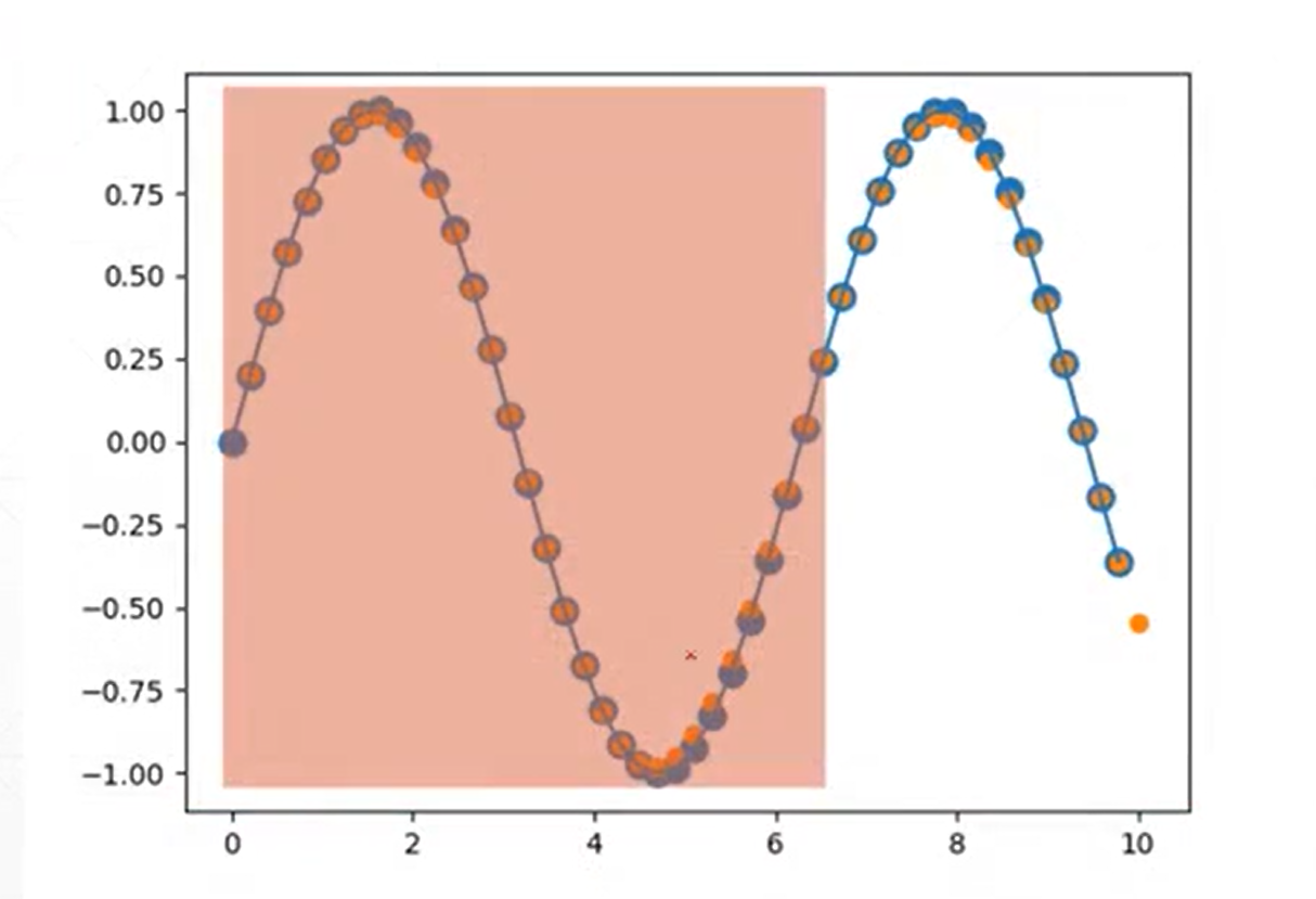
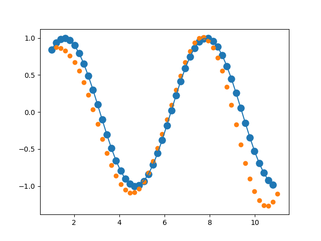
plt.scatter(time_steps[:-1], x.ravel(), s=90)
plt.plot(time_steps[:-1], x.ravel())
plt.scatter(time_steps[1:], predictions)
plt.show()
结果展示
LSTM代码讲解
简单回顾
源码
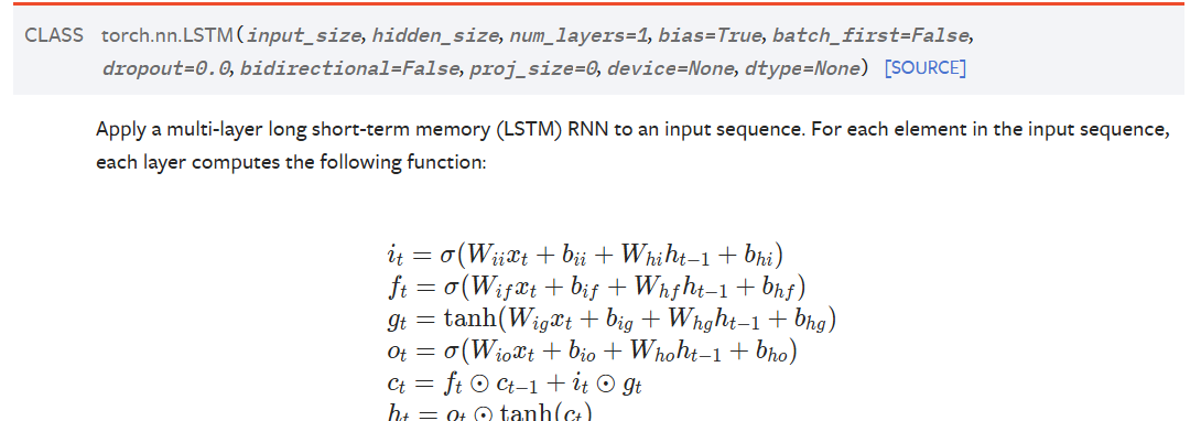
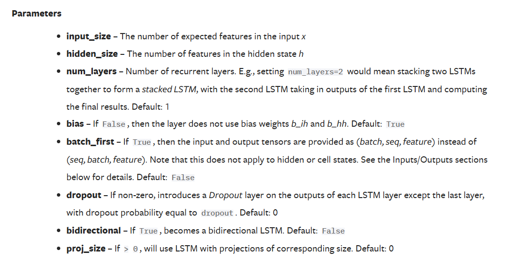
参数
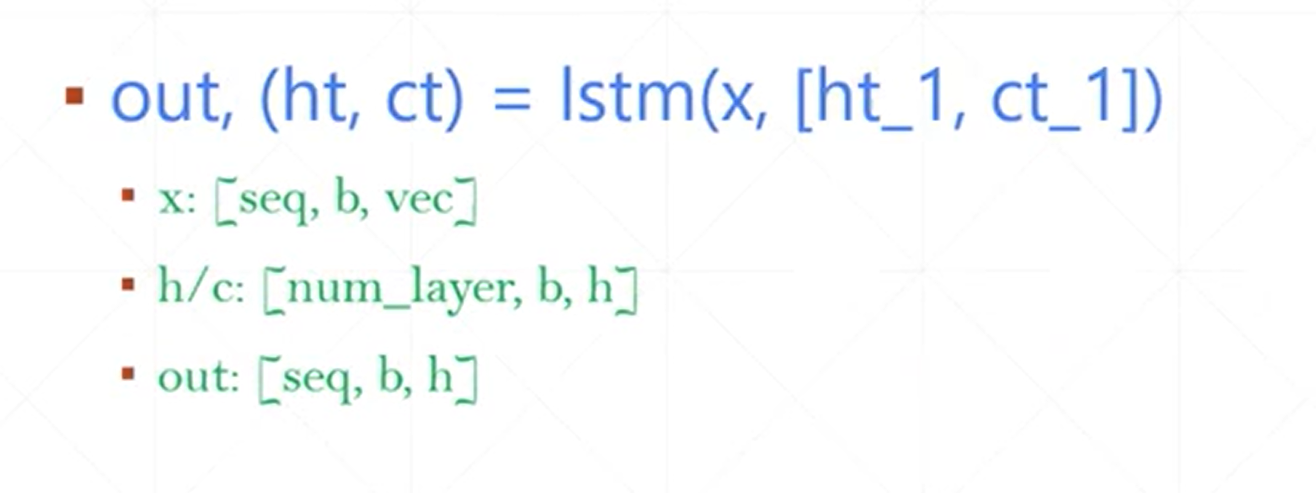
LSTM forward
示例代码
import torch
from torch import nn
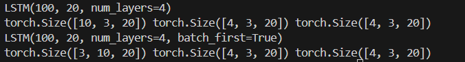
lstm = nn.LSTM(input_size=100, hidden_size=20, num_layers=4)
print(lstm)
x = torch.randn(10, 3, 100) # 10 seq, 3 batch, 100 dim
out, (h, c) = lstm(x)
print(out.shape, h.shape, c.shape)
lstm1 = nn.LSTM(input_size=100, hidden_size=20, num_layers=4, batch_first=True)
print(lstm1)
x = torch.randn(3, 10, 100) # 10 seq, 3 batch, 100 dim
out, (h, c) = lstm1(x)
print(out.shape, h.shape, c.shape)


 564
564

 被折叠的 条评论
为什么被折叠?
被折叠的 条评论
为什么被折叠?
 到【灌水乐园】发言


