


一、动态QCA实操代码粗略版
###五、QCA的拓展包setmethods可以用来处理面板数据
install.packages("SetMethods")#安装所需要的包

library(SetMethods)
data(SCHLF)
Head(SCHLF)

ttSL <- truthTable(SCHLF, conditions = "EMP, BARGAIN, UNI, OCCUP",
                    outcome ="EXPORT", incl.cut = .9, show,cases = TRUE)
sol_yi <- minimize(ttSL, include = "?", dir.exp = "0, 0, 0, 0")
cluster(results = sol_yi, data = SCHLF, outcome = "EXPORT",
        unit id ="COUNTRY", cluster id ="YEAR")

#第六条件的隶属度校准方法
?LR
#绘图查看数据DEV 为经济发展水平
Xplot(LR$DEV,at=pretty(LR$DEV),cex=0.8)
Xplot(LR$DEV,at=pretty(LR$DEV),cex = 0.8,jitter = TRUE)

#计算分类的门槛值
findTh(LR$DEV) ##使用聚类统计方法找到门槛值。此命令默认为两分类,故只有1个值
findTh(LR$DEV,n=3)#此命令网上,只是要求提出3个门槛值,即分为4类。

#分类/校准/新编码
recode(LR$DEV,rules="lo:550 =0;else =1")#一分二
calibrate(LR$DEV,type ="crisp",thresholds='550,850')#二分三
recode(LR$DEV,rules="lo:550=0;551:850=1;etse =2")#二分三
recode(LR$DEV,cuts="550,850",vaues =0:2)#二分三


##校准为模糊集的直接方法
recode(LR$DEV,cuts="350,550,850",values ="0,0.33,0.66,1")
LF$DEV #不同
#基于S形函数做校准
set.seed(12345)
height<-rnorm(n=100,mean=175,sd=10)#数据通常是正态分布的
range(height)
Xplot(height,cex=0.8,jitter = TRUE)
chidu1 <-calibrate(height,thresholds='e=165,c=175,i=185')#e代表完全不隶属;i代表完全隶属,c代表模糊值
chidu2 <-calibrate(height,thresholds='e=185,c=175,i=165')#与前一个反过来


#面图
par(mfrow=c(1,2),mai=c(0.6,0.9,0.8,0 .4))
plot(height,chidu1,main="a)隶属高个子集合的得分"xlab="身高cm",ylab="校准值,隶属于高个子的程度",col="red",cex=0.8)
plot(height,chidu2,main="b)隶属矮个子集合的得分",xlab="身高cm",ylab="校准值,隶属高个子的程度",col="blue",ce=0.8)


##可以调整上部分和下部分的弯曲程度
hsh1 <- calibrate(height,thresholds ="e=155,c=175,i=195",logistic = FALSE)#below 和 above 默认为1
hsh2 <- calibrate(height,thresholds ="e=155,c=175,i=195",logistic = FALSE,below = 2,above=2)
hsh3 <- calibrate( height,thresholds = "e=155,c=175.i=195", logstic   = FALSE, below=3.5, above =3.5)

plot(height,hsh3,cex = 0.6,col="yellow",main="三种校准函数的图形", xlab="身高 cm",ylab ="校准值")
points(height,hsh2,cex =0.6,col ="red")
points(height,hsh1,cex=0.6,col="green")


#又一个例子,国家收入
inc <-c(40110,34400,25200,24920,20060,17090,15320,13680,11720,11290,10940,9800,7470,4670,4100,4070,3740,3690,3590,2980,1000,650,450,110)
length(inc)
incal<-round(calibrate(inc,thresholds=c(2500,5000,20000)),2)


#间接校准,分两步
##第一步 用recoder()对数据重新编码
incr <- recode(inc,cuts="1000,4000,5000,10000,20000",values = seq(0,1,by=0.2))

##第二步数值转换借助回归等统计技术(分数多项式函数)
fracpol <-glm(incr~log(inc)+I(inc^(1/2))+I(inc^1)+I(inc^2),family= quasibinomial(logit))
round(predict(fracpol,type ="response"),3)
#预测值

##实际上上述两步可以由如下封装好的函数来完成
#cinc<- calibrate(inc,method ="indirect",thresholds="1000,4000,5000,10000,20000")round(cinc,3)

####定类数据只能校准为清晰集
####校准应该避免得出0.5的值来
######################################顺序变量的校准
#里克特式量表变量的校准:要7点以上,且值为均匀分布
##推荐使用基于等级顺序的方法TFR:
#generate artificial data
set.seed(12345)
values<- sample(1:7,100,replace =TRUE) ##从 1-7 中随机抽取 100 个数字,有放回。
E <- ecdf(values)
?ecdf
TFR <- pmax(0, (E(values)-E(1))/(1 -E(1)))
# the same values can be obtained via the embedded method:
TFR <- calibrate(values, method = "TFR" )
# The object TFR contains the fuzzy values obtained via this transformation:
table(round(TFR, 3))


##分类数据的校准方法(??)
set.seed(12345)
values <- sample(1:7,100,replace = TRUE)
E<-ecdf(values)##通过数据,推算出数据的累积函数,即推导出经验累积函数

TFR <- pmax(0,(E(values)-E(1)/(1-E(1))))
#构建TFR 方法,输出极大极小值
?pmax
##可以将TFR方法直接内化在校准函数里使用:
TFR <- calibrate(values,method="TFR")
table(round(TFR,3))#查看频次分布。
#round(value,3)保留3位小数


#####第七步必要条件分析
##必要条件集合X是结果集合Y的超集(相对于子集)
##与相关关系不同,集合关系不是对称的,因此需要分别对丫的存在和缺乏做必要性分析
##p113

LC$SURV
LC$DEV
with(Lc, table(SURV, DEV))
with(LC, sum(DEV & SURV)/sum(SURV))
########8/8

###直接计算必要条件的函数
pof("DEV","SURV",data=LC)
#或者
返回到标签页
pof("DEV<=SURV",data=LC)
##inclN 表示必要性的一致性指标;RON 表示必要性里的切题程度,covN 表示必要性的覆盖度;
##多值集合的必要条件计算
LM$DEV
POf("DEV{2}<=SURV",data=LM)#因为是多值,所以要分开来讨论
##同理,可以计算模糊集情况下必要条件的三个属性
pof("DEV<=SURV",data=LF)

###覆盖度与切题性的解释
#1 覆盖度
#如果X是Y的超集,而x比Y大得过多,则Y作为X的必要条件是缺少覆盖度的。
#p122
#2 切题性
#与覆盖度不一样,切题性是统计学思路,原理是卡方独立性检验
#如果一个事件的发生不发生不影响另外一件事情的发生概率,则两个变量是独立的。
#先确定必要条件的一致性程度,之后才能考量切题性。不能搞反了。


##比较几个条件的必要性程度
pof("DEV<=SURV",data=LF)
pof("LIT<=SURV",data=LF)
pof("URB<=SURV",data=LF)
#p130
XYplot(LIT, SURV, data= LF, jitter =TRUE, relation ="necessity")


######合取(交集)和析取(并集使用函数 fuzzygr())
##实际上可以采用一个简单的函数,一次性生成合取和析取的必要条件
superSubset(LF, outcome= "SURV", incl.cut = 0.9)

##结果给出了单个条件以及组合条件下的必要性三指标值,显示一致性的大于 0.9的结果
##再对切题度进行限定,让其不小于0.6
superSubset(LF,outcome="SURv",incl.cut=0.9,ron.cut =0.6)
二、动态QCA实操代码详细标注版
### 五、QCA的拓展包setmethods可以用来处理面板数据
# 安装并加载SetMethods包
install.packages("SetMethods")
library(SetMethods)

# 载入SCHLF数据集并查看前几行数据
data(SCHLF)
head(SCHLF)

# 基于SCHLF数据集进行truthTable分析
ttSL <- truthTable(SCHLF, conditions = "EMP, BARGAIN, UNI, OCCUP",
                   outcome = "EXPORT", incl.cut = 0.9, show.cases = TRUE)
sol_yi <- minimize(ttSL, include = "?", dir.exp = "0, 0, 0, 0")
cluster(results = sol_yi, data = SCHLF, outcome = "EXPORT",
        unit.id = "COUNTRY", cluster.id = "YEAR")

# 第六条件的隶属度校准方法
?LR

# 绘制DEV与经济发展水平相关的图表
Xplot(LR$DEV, at = pretty(LR$DEV), cex = 0.8)
Xplot(LR$DEV, at = pretty(LR$DEV), cex = 0.8, jitter = TRUE)

# 计算分类的门槛值
findTh(LR$DEV)  ## 使用聚类统计方法找到门槛值。此命令默认为两分类,故只有1个值
findTh(LR$DEV, n = 3)  # 此命令网上,只是要求提出3个门槛值,即分为4类。

# 分类/校准/新编码
recode(LR$DEV, rules = "lo:550 = 0; else = 1")  # 一分二
calibrate(LR$DEV, type = "crisp", thresholds = '550,850')  # 二分三
recode(LR$DEV, rules = "lo:550 = 0; 551:850 = 1; etse = 2")  # 二分三
recode(LR$DEV, cuts = "550,850", values = 0:2)  # 二分三

## 校准为模糊集的直接方法
recode(LR$DEV, cuts = "350,550,850", values = "0,0.33,0.66,1")
LF$DEV  # 不同

# 基于S形函数做校准
set.seed(12345)
height <- rnorm(n = 100, mean = 175, sd = 10)
range(height)
Xplot(height, cex = 0.8, jitter = TRUE)
chidu1 <- calibrate(height, thresholds = 'e=165,c=175,i=185')
chidu2 <- calibrate(height, thresholds = 'e=185,c=175,i=165')

# 面图
par(mfrow = c(1, 2), mai = c(0.6, 0.9, 0.8, 0.4))
plot(height, chidu1, main = "a)隶属高个子集合的得分", xlab = "身高cm", ylab = "校准值,隶属于高个子的程度", col = "red", cex = 0.8)
plot(height, chidu2, main = "b)隶属矮个子集合的得分", xlab = "身高cm", ylab = "校准值,隶属高个子的程度", col = "blue", cex = 0.8)

# 可以调整上部分和下部分的弯曲程度
hsh1 <- calibrate(height, thresholds = "e=155,c=175,i=195", logistic = FALSE)
hsh2 <- calibrate(height, thresholds = "e=155,c=175,i=195", logistic = FALSE, below = 2, above = 2)
hsh3 <- calibrate(height, thresholds = "e=155,c=175.i=195", logistic = FALSE, below = 3.5, above = 3.5)

plot(height, hsh3, cex = 0.6, col = "yellow", main = "三种校准函数的图形", xlab = "身高 cm", ylab = "校准值")
points(height, h
三、动态QCA实操代码
(一)学习资料
资料来源:面板数据QCA分析in R-03(软件操作)bilibili
###视频配套代码
###############面板数据的QCA分析操作(详细版)
#### setMethods()

1ibrary(setMethods)

# Import your clustered data in the long format.
# For example:
data(sCHLF)
str(SCHLF)

# Get the intermediate solution:
so1_yi <-minimize(SCHLF,outcome ="EXPORT",
                    conditions = ("EMP" ,“BARGAIN" ,"UNI" ,"OCCUP" ,"STOCK", “MA"),
                    inc1.cut =.9,
                    include ="?",
                    detai1s =TRUE,show.cases =TRuE,dir.exp =c(0,0,0,0,0,0))

# Get pooled, within, and between consistencies for the intermediate solution:
cluster(SCHLF,so1_yi,"EXPORT",unit_id ="COUNTRY",
        c1uster_id="YEAR",SOl =1)

#####
## or:
#c1uster(sCHLF, so1_yi,“EXPORT",
#        unit_id ="COUNTRY", c1uster_id="YEAR",so1 ="c1p1i1")

#必要条件分析
# Get pooled, within, and between consistencies for EMp as necessary for EXPORT:

c1uster(SCHLF, resuits="EMP", outcome="EXPORT", unit_id = "COUNTRY", c
        uster_id ="YEAR",necessity=TRUE)
###另外一种写法
## or:
#cluster(resu1ts=SCHLFSEMP, outcome=SCHLFSEXPORT, unit_id = SCHLFSCOUNTRY,
#        cluster_id =SCHLFSYEAR, necessity=TRUE)

######非“条件”的情况
# Get pooled, within, and between consistencies for ~EMp as necessary for EXPORT:
c1uster(SCHLF, resuits="~EMp", outcome="EXPORT", unit_id = "COUNTRY",
        c1uster_id ="YEAR", necessity=TRUE)

## or:
#cluster(resu1ts=1-SCHLF$EMP, outcome=SCHLF$EXPORT, unit_id = SCHLF$COUNTRY,
#        c1uster_id = SCHLF$YEAR, necessity=TRUE)


#########
#特定组态的充分条件分析
# Get pooled, within, and between consistencies for EMp*.MA*STocK as sufficient for
cluster(SCHLF,"EMP*~MA + ~STOCK","~EXPORT",unit_id ="COUNTRY",
        cluster_id ="YEAR")
# Get pooled, within, and between consistencies for EMp*MA + ~STocK as sufficient fc
c1uster(SCHLF,"EMP*MA + ~STOCK","~EXPORT",unit_id ="COUNTRY",
        cluster_id ="YEAR")

# Pot pooled,between,and within consistencies:
cluster.plot(cluster.res =so1_yi,
                TabS = TRUE,
                size =8,
                angle =6,
                wiconS = TRUE)
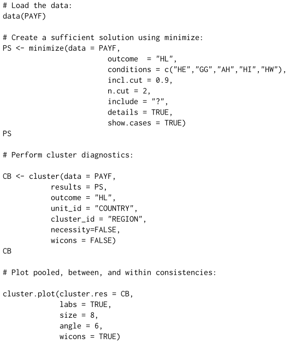
(二)修改后的实操代码
# 载入所需R包
library(SetMethods)

# 导入示例数据集sCHLF,并查看数据结构
data(SCHLF)
str(SCHLF)

##对未校准的数据进行校准,其中e代表完全不隶属;i代表完全隶属,c代表模糊值。
#chidu1 <-calibrate(height,thresholds='e=165,c=175,i=185')

# 找到中间解so1_yi,指定条件进行QCA分析
so1_yi <- minimize(SCHLF, outcome = "EXPORT",
                   conditions = c("EMP", "BARGAIN", "UNI", "OCCUP", "STOCK", "MA"),
                   inc1.cut = 0.9,
                   include = "?",
                   details = TRUE, show.cases = TRUE, dir.exp = c(0, 0, 0, 0, 0, 0))

# 对中间解进行一致性分析
cluster(sCHLF, so1_yi, "EXPORT", unit_id = "COUNTRY", cluster_id = "YEAR", SOl = 1)

# 对EMP作为必要条件进行一致性分析
cluster(sCHLF, results = "EMP", outcome = "EXPORT", unit_id = "COUNTRY", cluster_id = "YEAR", necessity = TRUE)

# 对非EMP情况进行一致性分析
cluster(sCHLF, results = "~EMP", outcome = "EXPORT", unit_id = "COUNTRY", cluster_id = "YEAR", necessity = TRUE)

# 针对特定组态条件进行充分条件分析
cluster(sCHLF, "EMP*~MA + ~STOCK", "~EXPORT", unit_id = "COUNTRY", cluster_id = "YEAR")

# 将结果以图表形式展示
cluster.plot(cluster.res = so1_yi,
             TabS = TRUE,
             size = 8,
             angle = 6,
             wicons = TRUE)
四、相关函数介绍
(1)SCHLF——(数据集)
SCHLF数据框架有76个观测值和9个变量。施耐德等人(2010)用来解释高科技产业资本多样性和出口绩效的数据。数据以长格式保存,前7个变量为模糊集。
EMP a numeric vector. Condition, employment protection.
EMP——一个数值向量。条件,雇佣保护。BARGAIN a numeric vector. Condition, collective bargaining.
BARGAIN——一个数值向量。条件,集体谈判。UNI a numeric vector. Condition, university training.
UNI——一个数值向量。条件,大学培训。OCCUP a numeric vector. Condition, occupational training.
OCCUP——一个数值向量。条件,职业培训。STOCK a numeric vector. Condition, stock market size.
STOCK——一个数值向量。条件,股市规模。MA a numeric vector. Condition, mergers and acquisitions.
MA——一个数值向量。条件,并购。EXPORT a numeric vector. Outcome, export performance in high-tech industries.
EXPORT——一个数值向量。结果,高科技产业的出口表现。COUNTRY a string vector. Name of the country in which the observation was made.
COUNTRY——一个字符串向量。观察所在国家的名称。YEAR a numeric vector. Year in which the observation was made.
YEAR——一个数值向量。观察所在年份。
(2)QCAradar—— Function for displaying a radar chart(显示雷达图的功能。)
描述:函数为“qca”类对象或布尔表达式显示雷达图。
使用:QCAradar(results, outcome= NULL, fit= FALSE, sol = 1)参数:result:一个qca类对象。要为否定结果执行充分解的雷达图,必须只使用从否定结果的充分性分析得到的最小化()结果。参数结果也可以是如下形式的布尔表达式:“a *~ b + ~ b * c”。
outcome:当结果类型为' qca '时,用大写字母表示结果名称的字符串。当为否定结果执行充分解的雷达图时,必须只使用从论证结果中否定结果的充分性分析得出的最小化()结果。不需要更改参数结果中的名称或使用波浪号。
fit—— Logical. Print parameters of fit when results is of type ’qca’(合乎逻辑的。当结果类型为“qca”时,打印拟合参数)
sol ——A vector where the first number indicates the number of the conservative or
parsimonious solution according to the order in the "qca" object. For more com-
plicated structures of model ambiguity, the intermediate solution can also be
specified by using a character string of the form "c1p3i2" where c = conserva-
tive solution, p = parsimonious solution and i = intermediate solution.(一个向量,其中第一个数字表示根据“qca”对象中的顺序的保守或简约解的个数。对于更复杂的模型模糊结构,也可以使用“c1p3i2”形式的字符串来指定中间解,其中c =保守解,p =简约解,i =中间解。)
案例:
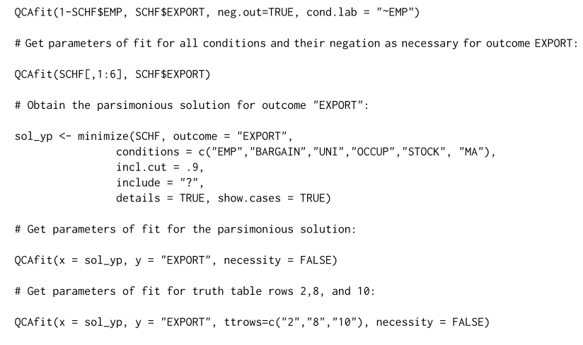
QCAfit(1-SCHF$EMP, SCHF$EXPORT, neg.out=TRUE, cond.lab = "~EMP")
# Get parameters of fit for all conditions and their negation as necessary for outcome EXPORT:
QCAfit(SCHF[,1:6], SCHF$EXPORT)
# Obtain the parsimonious solution for outcome "EXPORT":
sol_yp <- minimize(SCHF, outcome = "EXPORT",
conditions = c("EMP","BARGAIN","UNI","OCCUP","STOCK", "MA"),
incl.cut = .9,
include = "?",
details = TRUE, show.cases = TRUE)
# Get parameters of fit for the parsimonious solution:
QCAfit(x = sol_yp, y = "EXPORT", necessity = FALSE)
# Get parameters of fit for truth table rows 2,8, and 10:
QCAfit(x = sol_yp, y = "EXPORT", ttrows=c("2","8","10"), necessity = FALSE)
(3)xy.plot ——Function producing enhanced XY plots(生成增强型 XY 图的功能)
描述:xy。plot生成XY图形,并提供一致性、Haesebrouck一致性、覆盖率、RoN、PRI等值,多个图形参数可由用户自行决定。
它返回增强的XY图
使用:xy.plot(x, y, data, labcol = "black", main = "XY plot", ylab = "Outcome", xlab = "Condition", necessity = FALSE, jitter = FALSE, font = "sans", fontface = "italic", fontsize = 3, labs = rownames(data), crisp = FALSE, shape = 19, consH = FALSE, ...)参数:
x ——vector containing the condition.(包含条件的向量。)
y—— vector containing the outcome.(包含结果的向量。)
data ——The dataset used
labcol—— color of the dots.
main ——an overall title for the plot. The default is "XY plot". See ?title.(情节的总体标题。默认为“XY plot”。看到了什么?。)
ylab ——a title for the y-axis. The default is "Outcome". See ?title.(y轴标题,默认是输出)
xlab ——a title for the x-axis. The default is "Condition". See ?title.
necessity ——logical. Indicates if the parameters of fit are calculated for a sufficient or nec-
essary condition. The default is FALSE, therefore it calculates the parameters
of fit for sufficiency. To get the parameters of fit for necessary conditions set
necessity as TRUE.(合乎逻辑的。指示是否根据充分条件或必要条件计算拟合参数。默认值为FALSE,因此它计算适合的参数。为了获得必要条件的拟合参数,将必要性设为TRUE)
jitter ——Logical. Should labels be jitter to not overlap?(合乎逻辑的。标签是否应该抖动以避免重叠?)
font ——Font of the labels. Accepts "sans", "serif", and "mono" fonts.(标签字体。接受“sans”、“serif”和“mono”字体。)
fontface—— Fontface of the labels. Accepts "plain", "bold", "italic", "bold.italic".(标签的字体。接受"plain", "bold", "italic", "bold.italic"。)
fontsize—— Fontsize of the labels.(标签字体大小。)labs ——the vector of case labels. The default is the rownames of the dataset.(case标签的向量。默认值是数据集的行名。)
crisp ——Logical. Should a two-by-two table for crisp sets be returned?
shape ——The shape for the markers.(标记的形状。)
consH ——Logical. Should Haesebrouck’s consistency be printed?(合乎逻辑的。Haesebrouck的一致性应该被印出来吗?)
... Other internal arguments. Do not specify!
案例:
Examples
# Load the Schneider data:
data(SCHF)
# Plot of condition EMP as necessary for outcome EXPORT with case labels
# and names for the plot and axes:
xy.plot("EMP", "EXPORT", data=SCHF, necessity = TRUE,
main = "EMP as necessary for EXPORT", ylab = "EXPORT", xlab = "EMP")
(4)cluster——Diagnostic tool for clustered data.(聚类数据诊断工具。)
描述:该函数返回了类别为 "qca" 的对象和布尔表达式之间关系的汇总、内部一致性和外部一致性。
使用:cluster(data=NULL, results, outcome, unit_id, cluster_id, sol = 1, necessity = FALSE, wicons = FALSE)参数:
data A data frame in the long format containing both a colum with the unit names and a column with the cluster names. Column names should be in capital letters.
数据——一个长格式的数据框,包含单元名称和聚类名称。列名应大写。results An object of class "qca". For performing cluster diagnostics of the sufficient solution for the negated outcome one must only use the minimize() result from the sufficiency analysis of the negated outcome. The argument results can also be a vector, a character string, or a boolean expression of the form e.g. "A*~B + ~BC".
结果——一个类别为 "qca" 的对象。用于执行足够解的群集诊断时,必须仅使用 sufficiency analysis of the negated outcome 中的 minimize() 结果。参数 results 也可以是一个向量、一个字符字符串或一个布尔表达式,例如 "A~B + ~B*C"。outcome A character string with the name of the outcome in capital letters. When performing cluster diagnostics of the sufficient solution for the negated outcome one must only use the minimize() result from the sufficiency analysis of the negated outcome in the argument results. When performing cluster diagnostics for boolean expressions or vectors the negated outcome can be used by inserting a tilde in the outcome name in the argument outcome. The outcome can also be a vector.
结果变量——一个字符字符串,表示大写字母的结果变量的名称。在执行足够解的群集诊断时,必须仅使用结果中的 minimize() 结果。在执行布尔表达式或向量的群集诊断时,可以通过在结果变量名称中插入波浪符号来使用否定结果。结果变量也可以是一个向量。unit_id A character string with the name of the vector containing the units (e.g. coun-tries).
单位标识——一个字符字符串,表示包含单元(例如国家)的向量的名称。cluster_id A character string with the name of the vector containing the clustering units (e.g. years).
聚类标识——一个字符字符串,表示包含聚类单元(例如年份)的向量的名称。sol A vector where the first number indicates the number of the conservative or parsimonious solution according to the order in the "qca" object. For more complicated structures of model ambiguity, the intermediate solution can also be specified by using a character string of the form "c1p3i2" where c = conserva-tive solution, p = parsimonious solution and i = intermediate solution.
sol——一个向量,第一个数字表示与“qca” 对象中的顺序相对应的保守或简约解的编号。对于模型歧义结构更为复杂的情况,也可以通过使用形式为 "c1p3i2" 的字符字符串来指定中间解,其中 c = 保守解,p = 简约解,i = 中间解。cluster 7
聚类 7necessity Logical. Perform the diagnostic for the relationship of necessity?
必要性——逻辑值。是否执行必要性关系的诊断?wicons Logical. Should within consistencies and coverages be printed?
wicons——逻辑值。是否打印内部一致性和覆盖范围?
上述代码示例是用于执行群集分析(cluster diagnostics)的一系列命令。下面是对每个命令的解释:

1. 导入长格式的聚类数据:
```R
data(SCHLF)
```

2. 获取中间解(intermediate solution):
```R
sol_yi <- minimize(SCHLF, outcome = "EXPORT",
                conditions = c("EMP","BARGAIN","UNI","OCCUP","STOCK", "MA"),
                incl.cut = .9,
                include = "?",
                details = TRUE, show.cases = TRUE, dir.exp = c(0,0,0,0,0,0))
```

3. 获取中间解的汇总、内部一致性和外部一致性:
```R
cluster(SCHLF, sol_yi, "EXPORT", unit_id = "COUNTRY",
                cluster_id = "YEAR", sol = 1)
```
或者:
```R
cluster(SCHLF, sol_yi, "EXPORT", unit_id = "COUNTRY",
                cluster_id = "YEAR", sol = "c1p1i1")
```

4. 对于 EXPORT,获取 EMP 的汇总、内部一致性和外部一致性:
```R
cluster(SCHLF, results="EMP", outcome="EXPORT", unit_id = "COUNTRY",
                cluster_id = "YEAR", necessity=TRUE)
```
或者:
```R
cluster(results=SCHLF$EMP, outcome=SCHLF$EXPORT, unit_id = SCHLF$COUNTRY,
                cluster_id = SCHLF$YEAR, necessity=TRUE)
```

5. 对于 EXPORT,获取 ~EMP 的汇总、内部一致性和外部一致性:
```R
cluster(SCHLF, results="~EMP", outcome="EXPORT", unit_id = "COUNTRY",
                cluster_id = "YEAR", necessity=TRUE)
```
或者:
```R
cluster(results=1-SCHLF$EMP, outcome=SCHLF$EXPORT, unit_id = SCHLF$COUNTRY,
                cluster_id = SCHLF$YEAR, necessity=TRUE)
```

6. 对于 EXPORT,获取 EMP*~MA*STOCK 作为足够条件的汇总、内部一致性和外部一致性:
```R
cluster(SCHLF, "EMP*~MA*STOCK", "EXPORT", unit_id = "COUNTRY",
                cluster_id = "YEAR")
```

7. 对于 ~EXPORT,获取 EMP*MA + ~STOCK 作为足够条件的汇总、内部一致性和外部一致性:
```R
cluster(SCHLF, "EMP*MA + ~STOCK", "~EXPORT", unit_id = "COUNTRY",
                cluster_id = "YEAR")
```
(5)cluster.plot——Function for plotting pooled, between, and within consistencies for a cluster diagnostics.(用于绘制群集诊断的集合一致性、群集间一致性和群集内一致性的函数。)
描述:用于绘制群集诊断一致性池、一致性之间和一致性内部的函数。对于一个充分解,函数返回整个解和每个充分项的图。
使用:cluster.plot(cluster.res, labs = TRUE, size = 5, angle = 0, wicons = FALSE, wiconslabs = FALSE, wiconssize = 5, wiconsangle = 90)参数:
cluster.res An object of class "cluster.res". This is the result of a cluster diagnostics obtained with the cluster() function.
cluster.res——一个类别为 "cluster.res" 的对象。这是使用 cluster() 函数获取的群集诊断结果。labs Logical. Should labels for the clusters be printed?
labs——逻辑值。是否打印群集的标签?size Label font size for the clusters.
size——群集标签的字体大小。angle Label rotation for the clusters.
angle——群集标签的旋转角度。wicons Logical. Should within consistency plots be returned?
wicons——逻辑值。是否返回内部一致性图?wiconslabs Logical. Should labels for the units be printed?
wiconslabs——逻辑值。是否打印单位的标签?wiconssize Label font size for the units.
wiconssize——单位标签的字体大小。wiconsangle Label rotation for the units.
wiconsangle——单位标签的旋转角度。
案例:
(6)SetMethods-package ——Functions for Set-Theoretic Multi-Method Research and Advanced(集合理论多方法研究的功能和高级)QCA
描述:
这是作为C. Q. Schneider和C. Wagemann的《社会科学的集合理论方法》(剑桥大学出版社)一书的一个包的同伴而开始的。它现在已经发展到包括执行集合论多方法研究的功能(Schneider 2023, Schneider和Rohlfing 2013),聚类数据的QCA (Garcia-Castro和Arino 2013),理论评估,增强标准分析,QCA雷达图,间接校准,鲁棒性测试(Oana和Schneider - 2021)等。此外,它还包括复制Oana, i.e., C. Q. Schneider和E. Thomann的书中的例子的数据。使用R的定性比较分析(QCA):一个温和的介绍。剑桥大学出版社和C. Q. Schneider和C. Wagemann“社会科学的集合理论方法”,2021年,剑桥大学出版社。
该软件包包含集理论多方法研究、理论评估、聚类数据的QCA、增强标准分析、间接校准、计算拟合参数并生成XY图和QCA雷达图、执行鲁棒性测试等功能。
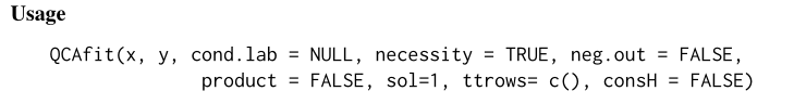
(7)QCAfit—— Function calculating the parameters of fit(函数计算参数的拟合)
描述:QCAfit是一种计算拟合参数的函数,适用于QCA和fsQCA,包括一致性、覆盖率、PRI、Haesebrouck一致性、RoN和PRODUCT。它适用于单一和多个条件。
使用:参数:
- x A vector containing the values of a condition, a matrix with more than one conditions, or an object of class "qca" when necessity is FALSE and when outcome is specified as a character string.
- x——包含条件值的向量,包含多个条件的矩阵,或当必要性为FALSE且outcome被指定为字符字符串时的“qca”类对象。(条件值的向量、包含多个条件的矩阵、或者在必要性为假且outcome被设定为字符字符串时的“qca”类对象)- y A vector containing the values of the output or a character string when y is of class "qca".
- y——包含输出值的向量或当y为“qca”类时的字符字符串。(包含输出值的向量或y为“qca”类时的字符字符串)- cond.lab When inserting a dataframe or a matrix with more than one condition and column names, the function automatically prints the names of the conditions tested. When inputting a vector, hence a single condition (i.e. a single column in a dataframe, the name of the condition tested should be inserted in this option.)
- cond.lab——在插入具有多个条件和列名的数据帧或矩阵时,函数会自动打印测试条件的名称。当输入向量时,因此单个条件(即数据框架中的单个列),应在此选项中插入已测试条件的名称。- necessity logical. It indicates if the output should be for sufficient or necessary condition(s). By default, FALSE, the function returns a table of parameters of fit for sufficient condition(s) (Consistency, Coverage, PRI, Haesebrouck’s Consistency, and optionally Product). When it set to TRUE the function returns a table of parameters of fit for necessary condition(s) (Consistency, Coverage, Relevance of Necessity).
- necessity——逻辑值。它指示输出是用于充分条件还是必要条件。默认值为FALSE,函数返回适合充分条件的拟合参数表格(一致性、覆盖率、PRI、Haesebrouck的一致性,可选择产品)。当设置为TRUE时,函数返回必要条件的拟合参数表格(一致性、覆盖率、必要性相关)。- neg.out logical. It indicates if the parameters of fit should be computed for the positive or the negative outcome. By default, FALSE, the function returns parameters of fit for the positive outcome.
- neg.out——逻辑值。它指示拟合参数是否应计算为正面或负面结果。默认值为FALSE,函数返回正面结果的拟合参数。- product logical. It indicates whether the parameter of fit PRODUCT should be shown. This stands for the product between the consistency sufficiency parameter and the PRI parameter.
- product——逻辑值。它指示是否应显示拟合参数PRODUCT。这代表一致性充分参数和PRI参数之间的乘积。- sol A vector where the first number indicates the number of the conservative or parsimonious solution according to the order in the "qca" object. For more complicated structures of model ambiguity, the intermediate solution can also be specified by using a character string of the form "c1p3i2" where c = conservative solution, p = parsimonious solution and i = intermediate solution.
- sol——一个向量,其中第一个数字表示根据“qca”对象中的顺序的保守或简约解决方案编号。对于更复杂的模型歧义结构,也可以使用"c1p3i2"形式的字符字符串指定中间解决方案,其中c = 保守解决方案,p = 简约解决方案,i = 中间解决方案。- ttrows A vector specifying the names of the truth table rows for which the function reports parameters of fit. For using this option y must be a "qca" object.
- ttrows——指定函数报告拟合参数的真值表行名称的向量。要使用该选项,y必须是一个“qca”对象。- consH Logical. Print also the Haesebrouck’s consistency among the parameters of fit?
- consH——逻辑值。是否也打印
案例: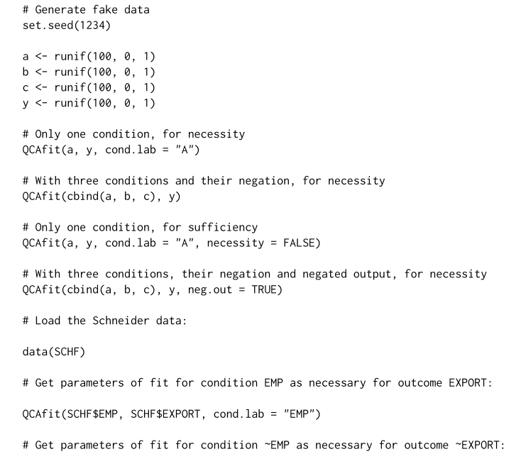
(8)calibrate——(校准函数。提取变量,并将其转换为因果和结果数据集的数值)
代码举例:
mtcars$mpg.fuzzy <- calibrate(mtcars$mpg,type="fuzzy",thresholds = c(10,20,30))
head(mtcars[,c("mpg","mpg.fuzzy")])
代码解释:
这段代码使用了R语言中的`calibrate`函数,将`mtcars`数据集中的`mpg`列进行模糊化处理,并将结果存储在新的列`mpg.fuzzy`中。以下是对这段代码的详细解释:

1. `mtcars$mpg.fuzzy <- calibrate(mtcars$mpg, type = "fuzzy", thresholds = c(10, 20, 30))`:
   - `mtcars$mpg`: 表示`mtcars`数据集中的`mpg`列,即汽车每加仑行驶的英里数。
   - `calibrate()`: 是一个函数,用于将原始数据模糊化处理。
   - `type = "fuzzy"`: 指定了模糊化的类型为“fuzzy”,表示对连续型的数据进行模糊化处理。
   - `thresholds = c(10, 20, 30)`: 定义了阈值,即划分模糊区域的界限。在这里,将`mpg`分成三个模糊区域:小于等于10,大于10且小于等于20,大于20且小于等于30,大于30。

2. `head(mtcars[,c("mpg","mpg.fuzzy")])`:
   - `head()`: R语言中的函数,用于显示数据框(data frame)的前几行。
   - `mtcars[,c("mpg","mpg.fuzzy")]`: 从`mtcars`数据集中选择`mpg`和`mpg.fuzzy`两列。

3.对calibrate函数中各参数的详细解释:
-x: 这是calibrate函数中的第一个参数,表示要进行模糊化处理的原始数据,通常是一个向量或数据框中的列(例如mtcars$mpg)。
-type: 这是calibrate函数的第二个参数,表示模糊化的类型。常见的类型包括:
"binary": 将连续变量转换为二元变量。
"fuzzy": 将连续变量模糊化处理,根据设定的阈值将其划分为不同的模糊区域。
-thresholds: 这是calibrate函数的第三个参数,用于指定阈值来划分模糊区域。对于模糊化处理,阈值通常以向量的形式提供。根据不同的阈值,数据会被划分为不同的模糊区域。
在我们之前的例子中,我们使用了type="fuzzy"来进行模糊化处理,并通过thresholds = c(10, 20, 30)来定义了三个阈值(10, 20, 30),将mpg列划分为小于等于10、大于10且小于等于20、大于20且小于等于30、大于30这四个模糊区域。

综上,这段代码的主要作用是将`mtcars`数据集中的`mpg`列进行模糊化处理,按照设定的阈值划分为不同的模糊区域,并将结果存储在新的列`mpg.fuzzy`中。最后,通过`head()`函数展示了`mpg`和`mpg.fuzzy`两列的前几行数据。
(9)truthTable——(创建真值表的函数)
示例代码:
truth<-truthTable(d.homeless,outcome="REP",
                  conditions=c("VI","DT","SA","CS","DF","PF"),
                  incl.cut1=0.8,
                  sort.by="incl")
详细解释:
##这段代码是用于生成一个逻辑相容性分析(Logical Consistency Analysis)的真值表(Truth Table)的功能。下面是对代码中的各部分进行详细解释:

- `truth <- truthTable(d.homeless, outcome="REP", conditions=c("VI","DT","SA","CS","DF","PF"), incl.cut1=0.8, sort.by="incl")`:
    - `d.homeless`: 这是传递给`truthTable`函数的数据集,其中包含了用于逻辑相容性分析的变量。

    - `outcome="REP"`: 指定了要分析的结果变量(outcome variable)为"REP",即根据何种条件来预测REP变量。

    - `conditions=c("VI","DT","SA","CS","DF","PF")`: 这里指定了作为条件的变量,它们是"VI"、"DT"、"SA"、"CS"、"DF"和"PF",用于逻辑相容性分析。

    - `incl.cut1=0.8`: 该参数表示只包括在真值表中出现频率至少为80%的情况。这有助于过滤掉低频的情况,提高真值表的可解释性。

    - `sort.by="incl"`: 这个参数指定了如何排序真值表中的行。在这种情况下,通过逻辑一致性的包含度(inclusivity)进行排序,以便更好地理解不同情况之间的关系。

    从整体上看,这段代码调用了`truthTable`函数来进行逻辑相容性分析,并生成一个真值表。真值表提供了不同条件下结果变量的组合情况及其频率,帮助用户了解不同条件之间的关系和逻辑一致性。排序参数使得结果更易于理解和解释。

##其余参数介绍,以下是一些常见的参数及其解释:
incl.cut2: 类似于incl.cut1,但指定了一个更高的阈值,只包括在真值表中出现频率至少为某一特定比例的情况。
min.cases: 指定每个条件组合至少需要有多少个案例才能被包括在真值表中。这有助于过滤掉样本较少的情况,确保结果的可靠性。
complexity: 控制生成真值表时考虑的条件组合的复杂性。可以是简单的布尔代数运算或更复杂的逻辑运算。
minimal: 控制是否生成最小化(minimal)的真值表,即在可能性保持不变的情况下尽量减少条件组合。
show.pm: 控制是否显示部分匹配(partial matches)的情况。部分匹配表示条件组合中有一些条件未满足的情况。
names.attr: 指定在真值表中显示的变量名称的属性。可以是变量的全名、缩写或其他形式。
通过灵活地调整这些参数,用户可以根据具体需求进行逻辑相容性分析,并生成符合要求的真值表。
五、配套享用资料
配套享用博主:QCA定性比较分析 in R 07 面板数据处理和必要条件分析
资源链接:https://pan.baidu.com/s/13_xhSn5gsvEs-6yNGR9D-A
提取码:nk(点赞、评论获取)鸣谢(对代码提出修改的):


 672
672

 被折叠的 条评论
为什么被折叠?
被折叠的 条评论
为什么被折叠?
 到【灌水乐园】发言


