


⛄一、获取代码方式
获取代码方式1:
完整代码已上传我的资源:【图像去噪】基于matlab全变分算法图像去噪【含Matlab源码 626期】
获取代码方式2:
付费专栏Matlab图像处理(初级版)
备注:
点击上面蓝色字体付费专栏Matlab图像处理(初级版),扫描上面二维码,付费29.9元订阅海神之光博客付费专栏Matlab图像处理(初级版),凭支付凭证,私信博主,可免费获得1份本博客上传CSDN资源代码(有效期为订阅日起,三天内有效);
点击CSDN资源下载链接:1份本博客上传CSDN资源代码
⛄二、图像去噪及滤波简介
1 图像去噪
1.1 图像噪声定义
噪声是干扰图像视觉效果的重要因素,图像去噪是指减少图像中噪声的过程。噪声分类有三种:加性噪声,乘性噪声和量化噪声。我们用f(x,y)表示图像,g(x,y)表示图像信号,n(x,y)表示噪声。
图像去噪是指减少数字图像中噪声的过程。现实中的数字图像在数字化和传输过程中常受到成像设备与外部环境噪声干扰等影响,称为含噪图像或噪声图像。去噪是图像处理研究中的一个重点内容。在图像的获取、传输、发送、接收、复制、输出等过程中,往往都会产生噪声,其中的椒盐噪声是比较常见的一种噪声,它属于加性噪声。
1.2 图像噪声来源
(1)图像获取过程中
图像传感器CCD和CMOS采集图像过程中受传感器材料属性、工作环境、电子元器件和电路结构等影响,会引入各种噪声。
(2)图像信号传输过程中
传输介质和记录设备等的不完善,数字图像在其传输记录过程中往往会受到多种噪声的污染。
1.3 噪声分类
噪声按照不同的分类标准可以有不同的分类形式:
基于产生原因:内部噪声,外部噪声。
基于噪声与信号的关系:
加性噪声:加性噪声和图像信号强度是不相关的,这类带有噪声的图像g可看成为理想无噪声图像f与噪声n之和:
g = f + n;
乘性嗓声:乘性噪声和图像信号是相关的,往往随图像信号的变化而变化,载送每一个象素信息的载体的变化而产生的噪声受信息本身调制。在某些情况下,如信号变化很小,噪声也不大。为了分析处理方便,常常将乘性噪声近似认为是加性噪声,而且总是假定信号和噪声是互相统计独立。
g = f + f*n
按照基于统计后的概率密度函数:
是比较重要的,主要因为引入数学模型这就有助于运用数学手段去除噪声。在不同场景下噪声的施加方式都不同,由于在外界的某种条件下,噪声下图像-原图像(没有噪声时)的概率密度函数(统计结果)服从某种分布函数,那么就把它归类为相应的噪声。下面将具体说明基于统计后的概率密度函数的噪声分类及其消除方式。
1.4 图像去噪算法的分类
(1)空间域滤波
空域滤波是在原图像上直接进行数据运算,对像素的灰度值进行处理。常见的空间域图像去噪算法有邻域平均法、中值滤波、低通滤波等。
(2)变换域滤波
图像变换域去噪方法是对图像进行某种变换,将图像从空间域转换到变换域,再对变换域中的变换系数进行处理,再进行反变换将图像从变换域转换到空间域来达到去除图像嗓声的目的。将图像从空间域转换到变换域的变换方法很多,如傅立叶变换、沃尔什-哈达玛变换、余弦变换、K-L变换以及小波变换等。而傅立叶变换和小波变换则是常见的用于图像去噪的变换方法。
(3)偏微分方程
偏微分方程是近年来兴起的一种图像处理方法,主要针对低层图像处理并取得了很好的效果。偏微分方程具有各向异性的特点,应用在图像去噪中,可以在去除噪声的同时,很好的保持边缘。偏微分方程的应用主要可以分为两类:一种是基本的迭代格式,通过随时间变化的更新,使得图像向所要得到的效果逐渐逼近,这种算法的代表为Perona和Malik的方程,以及对其改进后的后续工作。该方法在确定扩散系数时有很大的选择空间,在前向扩散的同时具有后向扩散的功能,所以,具有平滑图像和将边缘尖锐化的能力。偏微分方程在低噪声密度的图像处理中取得了较好的效果,但是在处理高噪声密度图像时去噪效果不好,而且处理时间明显高出许多。
(4)变分法
另一种利用数学进行图像去噪方法是基于变分法的思想,确定图像的能量函数,通过对能量函数的最小化工作,使得图像达到平滑状态,现在得到广泛应用的全变分TV模型就是这一类。这类方法的关键是找到合适的能量方程,保证演化的稳定性,获得理想的结果。
形态学噪声滤除器将开与闭结合可用来滤除噪声,首先对有噪声图像进行开运算,可选择结构要素矩阵比噪声尺寸大,因而开运算的结果是将背景噪声去除;再对前一步得到的图像进行闭运算,将图像上的噪声去掉。据此可知,此方法适用的图像类型是图像中的对象尺寸都比较大,且没有微小细节,对这类图像除噪效果会较好。
2 基于TV的图像去噪
2.1 TV图像去噪模型
全变分(TV) 图像去噪模型是由Rudin、Osher and Fatemi[4] 提出的, 并已成为图像去噪以及图像复原中最为成功的方法之一。TV图像去噪模型的成功之处就在于利用了自然图像内在的正则性,易于从噪声图像的解中反映真实图像的几何正则性,比如边界的平滑性15。
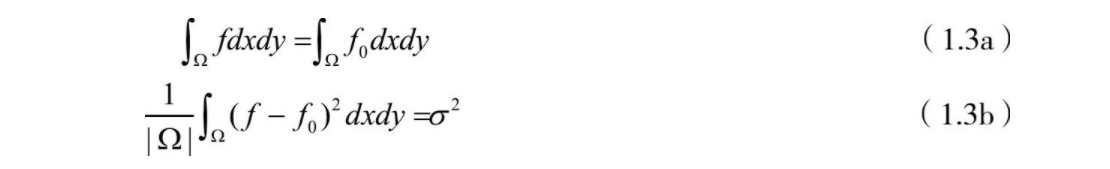
令f为原始的清晰图像,fo为被噪声污染的图像,即

式中n为具有零均值、方差为o²的随机噪声。Q表示图像的定义域,像素点(x,y)EΩ。通常有噪声图像的全变分比无噪声图像的全变分明显大,最小化全变分(TV)可以消除噪声,因此基于全变分的图像降噪可以归结为如下最小化问题:

满足约束条件:
最小化式 (1.2) 可以等价于最小化下式:
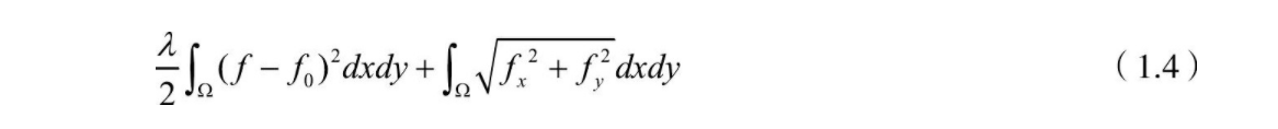
式中,第1项为数据保真项,它主要起保留原图像特性和降低图像失真度的作用;第2项为正则化项,参数为入规整参数,对平衡去噪与平滑起重要作用,它依赖于噪声水平。其导出的欧拉-拉格朗日方程为:

2.2 TV去噪的数值实现

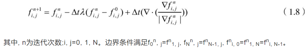
则求解方程 (1.5) 的离散迭代格式为:
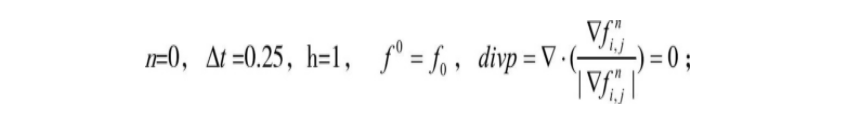
Step 1读入带噪图像f0;
Step 2初始化参数:

⛄三、部分源代码
function [img_estimated,energyi,ISNRi,energyo,ISNRo]=tvmm_debluring(img_noisy,h,lambda,varargin)
% function [img_estimated]=tvmm_debluring(img_noisy,h,lamdba,…
% ‘optional_parameter_name1’,value1,‘optional_parameter_name2’, value2,…);
%
% Total Variation-based image deconvolution with
% a majorization-minimization approach.
%
% Written by: Joao Oliveira, Jose Bioucas-Dias, Mario Figueiredo
% email: joao.oliveira@lx.it.pt
% SITE: www.lx.it.pt/~jpaos/tvmm
% Date: 21/11/2005
%
%
% ========================== INPUT PARAMETERS (required) =================
% Parameter Values
% name and description
% ========================================================================
% img_noisy (double) Noisy blured image of size ny.
% h (double) Blur kernel.
% lambda Regularization parameter (which is multiplied by the
% TV penalty).
%
% ======================== OPTIONAL INPUT PARAMETERS ====================
% Parameter Values
% name and description
% =======================================================================
% boa_iter (double) The number of outer loop iterations.
% Default: 20
% cg_iter (double) The max number of inner CG iterations.
% Default: 200
% soim_iter (double) The max number of inner SOIM iterations.
% Default: 20
% soim_cg_iter (double) The max number of CG iterations in inner SOIM.
% Default: 6
% cg_thrld (double) Conjugate Gradient threshold.
% Default: 1e-5;
% image (double) Original image.
% displayIm ({‘yes’,‘no’}) if ‘yes’ is passed the restored imaged
% is displayed along the CG iterations
% Default: ‘no’
% info_energyi ({‘yes’,‘no’}) if ‘yes’ is passed the isnr and energy of
% the objective function is displayed inside the inner loop.
% Default: ‘no’
% info_energyo ({‘yes’,‘no’}) if ‘yes’ is passed the energy of
% the objective function is displayed at each outter loop.
% Default: ‘no’
% info_ISNRi ({‘yes’,‘no’}) if ‘yes’ is passed the isnr is displayed.
% Default: ‘no’
% Requires: image
% info_ISNRo ({‘yes’,‘no’}) if ‘yes’ is passed the isnr is displayed.
% Default: ‘no’
% Requires: image
% x_0 (double) initial image iteration.
% Default: Wiener filter
% method ({‘cg’,‘soim’}) Selects the method used to solve the linear
% system: cg=conjugate gradient; soim=second order iterative
% method.
% Default: ‘cg’
% l_min (double) Minimum eigenvalue of the system for the second
% order iterative method.
% Default: 1e-5
% l_max (double) Maximum eigenvalue of the system for the second
% order iterative method.
% Default: 1
%
% ===================================================================
% The following functions can be provided in order to overwrite the
% internal ones. Recall that, by default, all calculations are
% performed with circular convolutions. (see Technical Report)
% ===================================================================
%
% mult_H (function_handle) Function handle to the function that
% performes Hx. This function must accept two parameters:
% x : image to apply the convolution kernel h
% h : Blur kernel
% mult_Ht (function_handle) Function handle to the function that
% performes Htx (Ht = H transpose). This function must
% accept two parameters:
% x : image to apply the convolution kernel h
% h : Blur kernel
% diffh (function_handle) Function handle to the function that
% computes the horizontal differences of an image x.
% diffv (function_handle) Function handle to the function that
% computes the vertical differences of an image x.
% diffht (function_handle) Function handle to the function that
% computes the horizontal differences (transposed) of an
% image x.
% diffh (function_handle) Function handle to the function that
% computes the vertical differences (transposed) of an
% image x.
%
%
% ====================== Output parameters ===============================
% img_estimated Estimated image
% energyi Energy of inner loop iterations.
% Required input arguments: ‘info_energyi’ and ‘image’.
% ISNRi Improvement Signal-to-noise ratio of inner loop iterations.
% Required input arguments: ‘info_ISNRi’ and ‘image’.
% energyo Energy of outer loop iterations.
% Required input arguments: ‘info_energyo’ and ‘image’.
% ISNRo Improvement Signal-to-noise ratio of outer loop iterations.
% Required input arguments: ‘info_ISNRo’ and ‘image’.
%
% ============= EXAMPLES =========================================
% Normal use:
% [img_estimated]=tvmm_debluring(img_noisy,lambda,sigma)
%
% Display restored images along CG iterations:
% [img_estimated]=tvmm_debluring(img_noisy,lambda,sigma,…
% ‘displayIm’,‘yes’)
%
% Perform ISNR calculations of the outer loop iterations:
% [img_estimated,energyi,ISNRi,energyo,ISNRo]=tvmm_debluring(img_noisy,…
% lambda,sigma,‘info_SNRo’,‘yes’,‘image’,image);
%
% ======================= DEFAULT PARAMETERS ===================
global mH mHt diffh diffv diffht diffvt
boa_iter = 20; % Number of outer loop iterations
cg_iter = 200; % Number of inner CG iterations
soim_iter = 20; % Number of inner SOIM iterations
soim_cg_iter = 6; % Number of CG iterations inside SOIM
cg_thrld = 1e-5; % CG threshold
displayIm = 0;
image=[];
info_energyi=‘no’;
info_energyo=‘no’;
info_ISNRi=‘no’;
info_ISNRo=‘no’;
info_int = 0;
info_ext = 0;
energyi=0;
ISNRi=0;
energyo=0;
ISNRo=0;
mH=@conv2c;
mHt=@conv2c;
diffh=@f_diffh;
diffv=@f_diffv;
diffht=@f_diffht;
diffvt=@f_diffvt;
method=‘cg’;
x_0=[];
l_min=1e-5;
l_max=1;
% ====================== INPUT PARAMETERS ========================
% Test for number of required parametres
if (nargin-length(varargin)) ~= 3
error(‘Wrong number of required parameters’);
end
% Read the optional parameters
if (rem(length(varargin),2)==1)
error(‘Optional parameters should always go by pairs’);
else
for i=1:2:(length(varargin)-1)
% change the value of parameter
switch varargin{i}
case ‘boa_iter’ % Outer loop iterations
boa_iter = varargin{i+1};
case ‘cg_iter’ % Inner loop iterations
cg_iter = varargin{i+1};
case ‘soim_iter’ % Inner loop iterations
soim_iter = varargin{i+1};
case ‘soim_cg_iter’ % CG iterations in Inner loop
soim_cg_iter = varargin{i+1};
case ‘displayIm’ % display sucessive xe estimates
if (isequal(varargin{i+1},‘yes’))
displayIm=1;
end
case ‘cg_thrld’ % CG threshold
cg_thrld = varargin{i+1};
case ‘image’ % Original image
image = varargin{i+1};
case ‘info_ISNRi’ % display ISNR inside inner loop
info_ISNRi = varargin{i+1};
case ‘info_ISNRo’ % display ISNR on outer loop
info_ISNRo = varargin{i+1};
case ‘info_energyi’ % display energy inside inner loop
info_energyi = varargin{i+1};
case ‘info_energyo’ % display energy on outer loop
info_energyo = varargin{i+1};
case ‘x_0’ % Initial image iteration
x_0 = varargin{i+1};
case ‘mult_H’ % Function handle to perform Hx
mH = varargin{i+1};
case ‘mult_Ht’ % Function handle to perform Htx
mHt = varargin{i+1};
case ‘diffh’ % External function to perform
diffh = varargin{i+1}; % horizontal differences
case ‘diffv’ % External function to perform
diffv = varargin{i+1}; % vertical differences
case ‘diffht’ % External function to perform
diffht = varargin{i+1}; % horizontal differences (transposed)
case ‘diffvt’ % External function to perform
diffvt = varargin{i+1}; % vertical differences (transposed)
case ‘method’ % External function to perform
method = varargin{i+1}; % vertical differences (transposed)
case ‘l_min’ % Minimum eigenvalue
l_min = varargin{i+1};
case ‘l_max’ % Maximum eigenvalue
l_max = varargin{i+1};
        otherwise
            % Hmmm, something wrong with the parameter string
            error(['Unrecognized parameter: ''' varargin{i} '''']);
    end;
end;
end
⛄四、运行结果


⛄五、matlab版本及参考文献
1 matlab版本
2014a
2 参考文献
[1]宋海英,荀月凤.全变分图像去噪的研究[J].成都电子机械高等专科学校学报. 2009,12(04)
3 备注
简介此部分摘自互联网,仅供参考,若侵权,联系删除


 335
335


 被折叠的 条评论
为什么被折叠?
被折叠的 条评论
为什么被折叠?
 到【灌水乐园】发言


