机器学习第一次上机报告

实验名称 实验1 机器学习模型评估实践 验证型
实验目的及要求：
1.掌握留出法、交叉验证法、自助法等数据集拆分方法；
2.掌握错误率、准确率、精确度、召回率、F1指标、真阳性率、假阳性率等指标的计算方法；
3.能够计算并绘制Precision-Recall（PR）曲线，并计算曲线下面积；
4.能够计算并绘制ROC曲线，并计算曲线下面积；
5.了解调用机器学习算法实现算法性能评估及预测的基本流程。
实验内容：
【实验项目1】
(1) 利用python或matlab实现“留出法” 拆分数据集；
(2) 利用python或matlab实现“交叉验证法”拆分数据集；
(3) 利用python或matlab实现“自助法”拆分数据集。
注：自行随机生成数据集（特征+标签），或调用scikit-learn内置数据集。

【实验项目2】
(1) 利用python或matlab实现“错误率”、 “准确率” 指标的计算；
(2) 利用python或matlab实现“精确度” 、“召回率” 、“F1”指标的计算， 并绘制Precision-Recall（PR）曲线，计算曲线下面积；
(3) 利用python或matlab实现“真阳性率” 、“假阳性率”指标的计算,并绘制ROC曲线，计算曲线下面积。
注：可自行生成预测分值列表和标签列表用于测试代码，或调用scikit-learn内置数据集和预测方法。

【实验项目3】
(1) 尝试利用python或matlab，采用“交叉验证”或者其它方式，评估机器学习算法的性能，了解评估流程。

参考教材资料
《机器学习》，周志华，清华大学出版社，2016年
sklearn模型选择和评估 https://www.scikitlearn.com.cn/0.21.3/30/

实验考核材料
（1）实验报告：按实验内容及任务要求，记录各项任务的关键步骤和截屏；
（2）代码脚本：保存完整的执行脚本。
将所有材料打包，提交到作业系统。

操作步骤：
这里我使用非常著名的新手数据集mnist。为了示范简单的深度学习训练（机器学习的一个非常大分支，能达到的效果和传统机器学习是一样的）、评估的完整流程，我从mnist测试集入手，不使用类似datasets.MNIST的接口，从而使得这套流程可以套用你自己的分类数据集。因为是分类任务，我直接将类别嵌入文件名，这样对图片进行处理的同时，类别标签也得到了处理。另外，本实验尽量没有使用框架，如果你是新手，弄懂这一套流程你会大受裨益！
有人反馈说运行不了，很大原因是你环境没配好，这个需要你百度、csdn自己配一下，实在配不好的可以评论区提问，我看到会回答的，其他问题也可以提，环境配好，文件目录改一下，文末的压缩包代码基本是肯定可以运行的，环境还是配置好，后续实验我应该会更新的，本次所需要的功能库如下：
必须的：
torch和torchvision可以安装gpu版本或者cpu版本，看你电脑是否有英伟达显卡

import random
import shutil
from glob import glob
import os
import numpy as np
from matplotlib import pyplot as plt
import cv2
#以下只需要安装torch就行
from torch.nn.functional import cross_entropy
import torch
from torch import nn
from torch.utils.data import DataLoader
from torch.utils.data import Dataset
#安装torchvision就行了
from torchvision.models import resnet18
import torchvision.transforms as tf

非必需：（只是可以查看进度与屏蔽一些多余的警告）

from tqdm import tqdm
import warnings

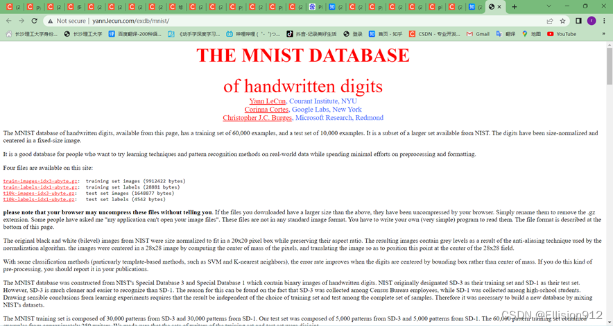
1. 在官网下载数据集（下载链接：http://yann.lecun.com/exdb/mnist/）
   

2. 然后我们需要把它转化成图片格式

def byte2img():
    import numpy as np
    import struct

    from PIL import Image
    import os

    dataset_path = './'  # 需要修改的路径:解压的数据集所在文件夹
    data_file = dataset_path + 't10k-images.idx3-ubyte'

    # It's 7840016B, but we should set to 7840000B
    data_file_size = 7840016
    data_file_size = str(data_file_size - 16) + 'B'

    data_buf = open(data_file, 'rb').read()

    magic, numImages, numRows, numColumns = struct.unpack_from('>IIII', data_buf, 0)
    datas = struct.unpack_from('>' + data_file_size, data_buf, struct.calcsize('>IIII'))
    datas = np.array(datas).astype(np.uint8).reshape(numImages, 1, numRows, numColumns)

    label_file = dataset_path + 't10k-labels.idx1-ubyte'

    # It's 10008B, but we should set to 10000B
    label_file_size = 10008
    label_file_size = str(label_file_size - 8) + 'B'

    label_buf = open(label_file, 'rb').read()

    magic, numLabels = struct.unpack_from('>II', label_buf, 0)
    labels = struct.unpack_from('>' + label_file_size, label_buf, struct.calcsize('>II'))
    labels = np.array(labels).astype(np.int64)

    test_path = dataset_path + 'mnist_test'
    if not os.path.exists(test_path):
        os.mkdir(test_path)

    # 新建 0~9 十个文件夹，存放转换后的图片
    for i in range(10):
        file_name = test_path + os.sep + str(i)
        if not os.path.exists(file_name):
            os.mkdir(file_name)

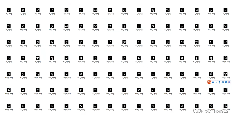
    for ii in range(numLabels):
        img = Image.fromarray(datas[ii, 0, 0:28, 0:28])
        label = labels[ii]
        file_name = test_path + os.sep + str(label) + os.sep + str(ii) + '_' + str(label) + '.png'#类别嵌入文件名
        img.save(file_name)

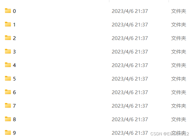
类别嵌入文件名：

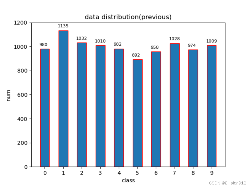
划分前数据分布情况：

def plot(x_value,title):#画图
    fig=plt.figure()
    nums, bins, patches=plt.hist(x_value, bins=10,edgecolor="r",rwidth=0.5,align='left',range=(0,10))
    y_max=int(max(nums))+100
    plt.ylim((0,y_max))
    for x in range(10):
        plt.text(bins[x]-0.3 , nums[x]+int(y_max/30), int(nums[x]),  va='top',color='k', fontsize=8)
    plt.xticks(range(10))
    plt.title(title)
    plt.xlabel("class")
    plt.ylabel("num")
    plt.savefig('./'+str(y_max)+'.png')
    plt.close(fig)
def analyse():#分析数据分布
    data_dir=r'C:\Users\River\Desktop\dataset\mnist_test\*'
    data_distribution_lst=[]
    for i,class_dir in enumerate(glob(data_dir)):
        data_file=os.listdir(class_dir)
        nums=int(len(data_file))
        class_num=[i]*nums
        data_distribution_lst+=class_num
    plot(data_distribution_lst)

【实验项目1】
(4) 利用python或matlab实现“留出法” 拆分数据集；
原理：留出法：直接将数据集D划分为两个互斥的集合，一个作为训练集S，另一个作为测试集 T，即 D=S∪T，S∩T=∅。
说明：
（a）测试集合和训练集合尽可能保持数据分布的一致性，比如要保证正反样本的比例不变（这是一种导致过拟合的原因）；
（b）在给定了训练/测试集合的样本比例之后，仍要存在多种的划分方式，对数据集合D进行分割（单次使用留出法结果往往不够稳定）；
（c）训练/测试集合的大小比例问题；
测试集合过小，会导致测评结果的方差变大；
训练集合过小，会导致偏差过大，一般使用的都是2/3~4/5的样本用于训练
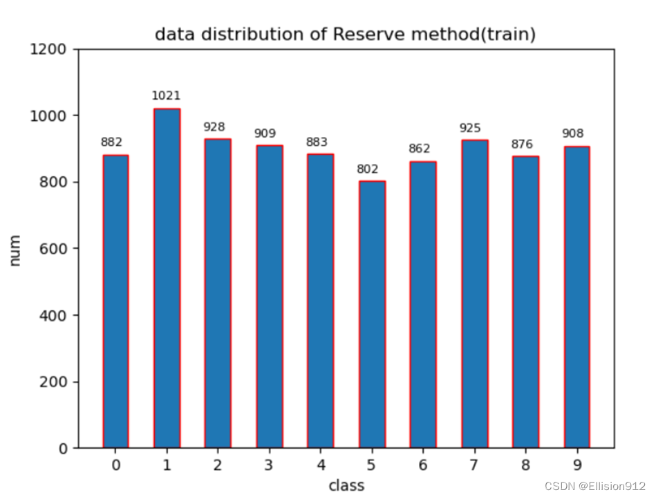
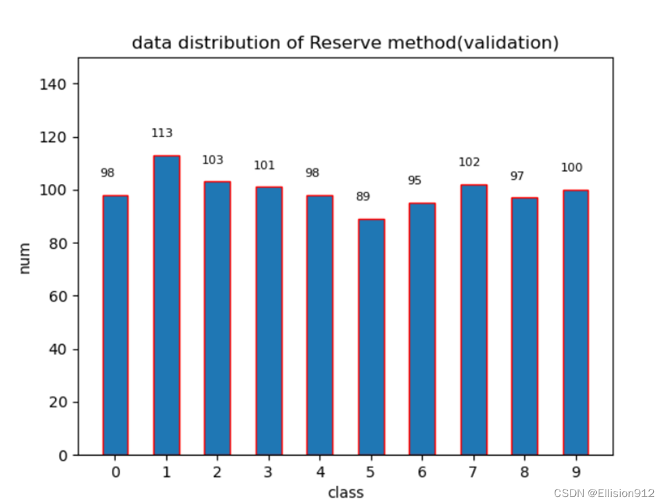
按9：1划分数据分布情况：

def move_file(rate=0.9):#留出法
    data_dir=r'C:\Users\River\Desktop\dataset\mnist_test\*'#原数据目录
    train_dir=r'C:\Users\River\Desktop\dataset\mnist_test\train'#划分后训练数据目录
    test_dir=r'C:\Users\River\Desktop\dataset\mnist_test\test'#划分后测试数据目录
    for class_dir in tqdm(glob(data_dir)):#分层抽样
        file_name_=os.path.join(class_dir,'*.png')
        file_lst=glob(file_name_)
        random.shuffle(file_lst)#随机打乱
        nums=int(len(file_lst)*rate)
        train_lst=file_lst[:nums]
        test_lst=file_lst[nums:]
        for img_path in train_lst:
            shutil.copy(img_path,train_dir)
        for img_path in test_lst:
            shutil.copy(img_path,test_dir)

(5) 利用python或matlab实现“交叉验证法”拆分数据集；
原理：交叉验证法:随机将样本拆分成K个互不相交大小相同的子集，然后用K-1个子集作为训练集训练模型，用剩余的子集测试模型，对K中选择重复进行，最终选出K次测评中的平均测试误差最小的模型
说明：
（a）假设我们确定了折数k，由于进行划分的方法不同，得到的结果也会不同（例如使用不同的随机数种子）。在实际使用中，我们可以进行 p次不同的k折交叉验证，取p*k 次实验结果的平均作为最终的实验结果，这叫做p次k折交叉验证。例如，10次10折交叉验证共进行了100次实验。
（b）与留出法类似，划分为S折存在多种方式，所以为了减小样本划分不同而引入的误差，通常随机使用不同的划分重复P次，即为P次S折交叉验证

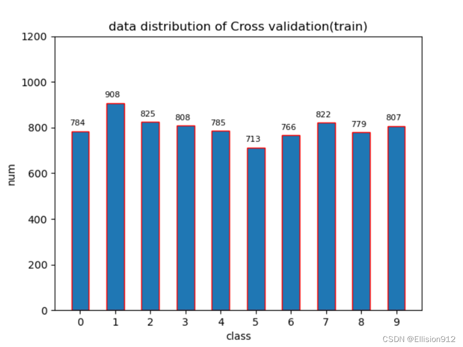
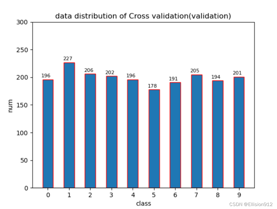
5折交叉数据分布情况（第一折交叉）：

def k_fold(k):#k折交叉验证
    data_dir=r'C:\Users\River\Desktop\dataset\mnist_test\*'
    train_dir=r'C:\Users\River\Desktop\dataset\mnist_test\train\*'
    test_dir=r'C:\Users\River\Desktop\dataset\mnist_test\test\*'
    for class_dir in tqdm(glob(data_dir)):#分层抽样
        file_name_=os.path.join(class_dir,'*.png')
        file_lst=glob(file_name_)
        random.shuffle(file_lst)#随机打乱
        nums=len(file_lst)//k
        for i, tt_path in enumerate(zip(glob(train_dir),glob(test_dir))):#移动数据
            train_path=tt_path[0]
            test_path=tt_path[1]
            lft=nums*i
            rt=nums*(i+1)
            train_lst=file_lst[:lft]+file_lst[rt:]
            test_lst=file_lst[lft:rt]
            for img_path in train_lst:
                shutil.copy(img_path,train_path)
            for img_path in test_lst:
                shutil.copy(img_path,test_path)

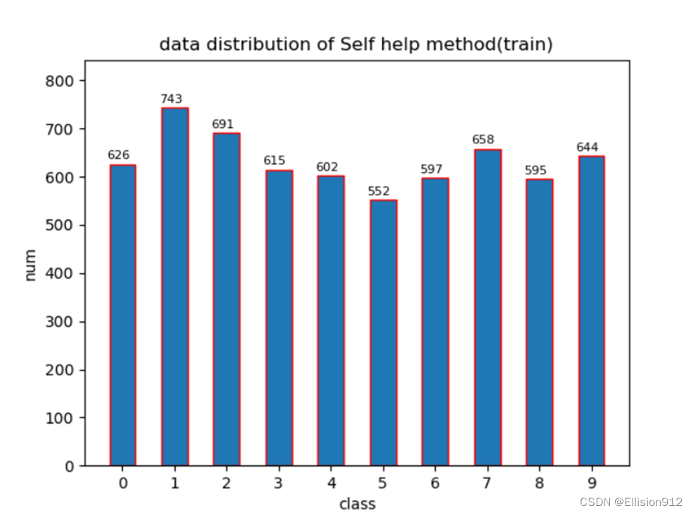
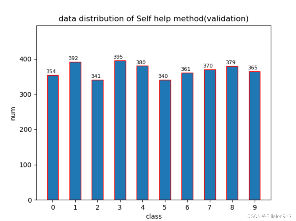
(6) 利用python或matlab实现“自助法”拆分数据集。
注：自行随机生成数据集（特征+标签），或调用scikit-learn内置数据集。
原理：自助法：留出法每次从数据集 D 中抽取一个样本加入数据集 D′ 中，然后再将该样本放回到原数据集 D 中，即 D 中的样本可以被重复抽取。这样，D 中的一部分样本会被多次抽到，而另一部分样本从未被抽到。假设抽取 m 次，则在 m 次抽样中都没有被抽到的概率为 (1−1/m)m，取极限有：
也就是说，原数据集 D 中约 36.8% 的数据未在 D′ 中出现过，所以我们可以将 D′ 作为训练集，将 D−D′（D 与 D′ 的差集）作为测试集。
说明：自助法适用于数据集较小，难以划分训练、验证集的情况。

def Self_help_method():#自助法
    data_dir = r'mnist_test\*'
    train_dir = r'train'
    test_dir = r'test'
    file_lst = []
    train_lst = []
    for class_dir in tqdm(glob(data_dir)):  # 得到所有文件绝对路径
        file_name_ = os.path.join(class_dir, '*.png')
        file_lst += glob(file_name_)
    sum_nums = len(file_lst)
    for i in range(sum_nums):  # 进行sum_nums次抽取
        train_lst.append(file_lst[int(random.random() * sum_nums)])
    train_lst = set(train_lst)  # 去除重复
    test_lst = set(file_lst).difference(train_lst)  # 求集合差集得验证集
    train_value = []
    test_value = []
    for img_path in train_lst:
        # train_value.append(int(img_path.split('\\')[6]))
        shutil.copy(img_path, train_dir)
    for img_path in test_lst:
        # test_value.append(int(img_path.split('\\')[6]))
        shutil.copy(img_path, test_dir)

抽取10000次（数据集数量为10000张）的数据分布情况：


【实验项目2】
不涉及PR、ROC曲线时，本实验根据预测和标签直接构造混淆矩阵（不懂的建议自行百度，非常重要），然后直接计算各种指标（对数组结果直接取平均）
混淆矩阵：

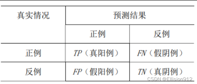
TP 表示正确分出正例的数量；FN 表示把正例错分为反例的数量；TN 表示正确分出反例的数量；
FP表示把反例错分为正例的数量
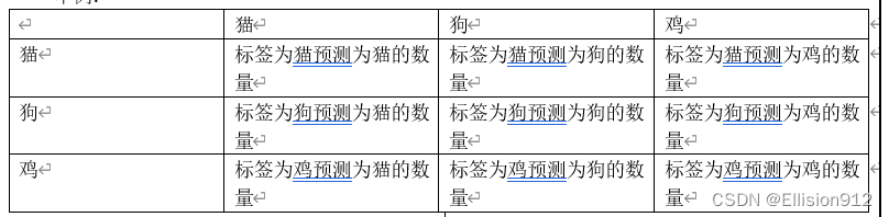
举例：

求混淆矩阵以及下述要求的各种指标代码：

class SegmentationMetric(object):
    def __init__(self, numClass):
        self.numClass = numClass
        self.confusionMatrix = np.zeros((self.numClass,) * 2)
    def genConfusionMatrix(self, imgPredict, imgLabel):  # 同FCN中score.py的fast_hist()函数
        # remove classes from unlabeled pixels in gt image and predict
        mask = (imgLabel >= 0) & (imgLabel < self.numClass)
        label = self.numClass * imgLabel[mask] + imgPredict[mask]
        count = np.bincount(label, minlength=self.numClass ** 2)
        confusionMatrix = count.reshape(self.numClass, self.numClass)
        return confusionMatrix

    def addBatch(self, imgPredict, imgLabel):
        assert imgPredict.shape == imgLabel.shape
        self.confusionMatrix += self.genConfusionMatrix(imgPredict, imgLabel)

    def reset(self):
        self.confusionMatrix = np.zeros((self.numClass, self.numClass))

    def Accuracy(self):#准确率
        #  PA = acc = (TP + TN) / (TP + FN + FP + TN)
        acc = np.diag(self.confusionMatrix).sum() / self.confusionMatrix.sum()
        error_rate=1-acc#错误率
        return acc,error_rate

    def Precision(self):
        # return each category pixel accuracy(A more accurate way to call it precision)
        # acc = (TP) / (TP + FP)
        precision = np.diag(self.confusionMatrix) / self.confusionMatrix.sum(axis=0)
        return np.nanmean(precision)  

    def F1(self):
        # F1 = (2*recall*precision) / (recall+precision)
        f1 = (2*self.Recall()*self.Precision())/(self.Recall()+self.Precision())
        return f1


    def Recall(self):
        # recall = (TP) / (TP + FN)
        recall = np.diag(self.confusionMatrix) / self.confusionMatrix.sum(axis=1)
        return np.nanmean(recall)

    def FPR(self):
        # recall = (FP) / (FP + TN)
        FP=self.confusionMatrix.sum(axis=0)-np.diag(self.confusionMatrix)
        FP_TN=np.repeat(self.confusionMatrix.sum(),self.numClass)-np.sum(self.confusionMatrix, axis=1)
        fpr = FP/FP_TN
        return np.nanmean(fpr)

(4) 利用python或matlab实现“错误率”、 “准确率” 指标的计算；
准确率 = (TP + TN) / (TP + FN + FP + TN)
错误率=1-准确率
(5) 利用python或matlab实现“精确度” 、“召回率” 、“F1”指标的计算， 并绘制Precision-Recall（PR）曲线，计算曲线下面积；
精确度= (TP) / (TP + FP)
召回率= (TP) / (TP + FN)
F1= (2召回率精确度) / (召回率+精确度)
绘制曲线：
以这实验为例（10分类），由模型计算得到置信度矩阵（[*,10]），从中依次取不同的数作为阈值，以某个图片预测为例，它有10个预测概率，当第0个概率值大于等于阈值（数组从0开始），同时标签又为0时（假设为0），那么0这个类别的TP+1，若第1个概率值大于等于阈值，此时标签对不上就FP+1；同理，概率值小于阈值，标签对上，FN+1，或者标签对不上就TN+1，类似地依次进行。 再根据精确度，召回率公式求出其坐标
最终一个阈值就可以确定一组P-R值作为坐标，注意PR必过（0，1）点。最后将其画出即可
可以将曲线（其实是折线）下的多边形分割成多个直角梯形求面积
(6) 利用python或matlab实现“真阳性率” 、“假阳性率”指标的计算,并绘制ROC曲线，计算曲线下面积。
注：可自行生成预测分值列表和标签列表用于测试代码，或调用scikit-learn内置数据集和预测方法。
真阳性率= TP / ( TP+FN )
假阳性率= FP / ( FP + TN )
和PR曲线绘制同理，注意ROC曲线必过（0，0）、（1，1）两点
面积与（5）同理

绘制曲线以及计算面积代码：

def cal_S(macro_recall, macro_precis):  # 划分为小梯形计算
    S = .0
    x_l, y_l = macro_recall[0], macro_precis[0]
    for x_r, y_r in zip(macro_recall[1:], macro_recall[1:]):
        S += (y_l + y_r) * (x_r - x_l) / 2
    print(S)


def plot(xlabel, ylabel, title, x, y):
    fig = plt.figure()
    plt.xlim([-0.01, 1.01])
    plt.ylim([-0.01, 1.01])
    plt.xlabel(xlabel)
    plt.ylabel(ylabel)
    plt.title(title)
    plt.plot(x, y)
    plt.savefig('./' + title + '.png')
    plt.close(fig)


def cal_plot_pr_roc(num_classes=10, score_path="./net_out.txt.txt"):
    with open(score_path, 'r') as f:
        files = f.readlines()  # 读取文件

    macro_precis = []
    macro_recall = []
    macro_FPR = [0]

    lis_all = []
    for file in tqdm(files):
        a = file.strip().split(" ")
        lis_all += a[1:]
    lis_order = sorted(set(lis_all))  # 记录所有得分情况，并去重从小到大排序，寻找各个阈值点

    for i in tqdm(lis_order[::100]):  # 每100个点取一个阈值,数越大，迭代次数越少，速度越快，但图的精度会降低

        true_p = np.zeros(num_classes)  # 真阳
        true_n = np.zeros(num_classes)  # 真阴
        false_p = np.zeros(num_classes)  # 假阳
        false_n = np.zeros(num_classes)  # 假阴

        for file in files:
            file_c = file.strip().split(" ")  # 分别计算比较各个类别的得分，分开计算，各自为二分类
            # 最后求平均，得出宏pr
            for j in range(num_classes):

                if float(file_c[j + 1]) >= float(i) and int(file_c[0]) == j:  # 遍历所有样本，第0类为正样本，其他类为负样本，
                    true_p[j] = true_p[j] + 1  # 大于等于阈值，并且真实为正样本，即为真阳，
                elif float(file_c[j + 1]) >= float(i) and int(file_c[0]) != j:  # 大于等于阈值，真实为负样本，即为假阳；
                    false_p[j] = false_p[j] + 1  # 小于阈值，真实为正样本，即为假阴
                elif float(file_c[j + 1]) < float(i) and int(file_c[0]) == j:
                    false_n[j] = false_n[j] + 1
                else:
                    true_n[j] = true_n[j] + 1
        prec = np.zeros(num_classes)
        recall = np.zeros(num_classes)
        FPR = np.zeros(num_classes)
        for j in range(num_classes):
            prec[j] = (true_p[j] + 0.00000000001) / (true_p[j] + false_p[j] + 0.00000000001)
            recall[j] = (true_p[j] + 0.00000000001) / (true_p[j] + false_n[j] + 0.00000000001)
            FPR[j] = (false_p[j] + 0.00000000001) / (true_n[j] + false_p[j] + 0.00000000001)  # 计算各类别的召回率，小数防止分母为0

        precision = prec.mean()
        recall = recall.mean()  # 多分类求得平均精确度和平均召回率，即宏macro_pr
        FPR = FPR.mean()
        macro_FPR.append(FPR)
        macro_precis.append(precision)
        macro_recall.append(recall)

    # 添加必过点
    macro_FPR.append(1)
    TPR = macro_recall.copy()#一定要copy,直接赋值往往会因为变量名的原因重复操作
    TPR.insert(0, 0)
    TPR.append(1)
    macro_precis.append(1)
    macro_recall.append(0)

    # 保证顺序以形成一个函数曲线
    z = list(zip(macro_recall, macro_precis))
    roc = list(zip(macro_FPR, TPR))
    z = sorted(z)
    roc = sorted(roc)
    macro_recall, macro_precis = zip(*z)
    macro_FPR, TPR = zip(*roc)
    x, y = np.array(macro_recall), np.array(macro_precis)
    roc_x, roc_y = np.array(macro_FPR), np.array(TPR)

    # 计算面积
    print('PR_S:')
    cal_S(x, y)
    print('ROC_S:')
    cal_S(roc_x, roc_y)

    # 画图
    plot(xlabel='recall', ylabel='precision', title='PR_curve', x=x, y=y)
    plot(xlabel='FPR', ylabel='TPR', title='ROC_curve', x=roc_x, y=roc_y)

【实验项目3】
(7) 尝试利用python或matlab，采用“交叉验证”或者其它方式，评估机器学习算法的性能，了解评估流程。
本实验采用自助法划分训练集验证集（最好采用交叉验证，说服力最高），像大部分机器学习实验一样，不再单独划分测试集。分别使用pytorch框架自带的resnet18模型和我自己设计的微小模型进行训练，评估。实验平台window10，GPU 3080Ti（这种微小数据集cpu也能跑）

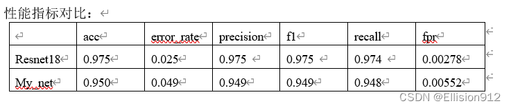
从图中可以看出resnet18的准确率和查全率都很高（f1可以说明）

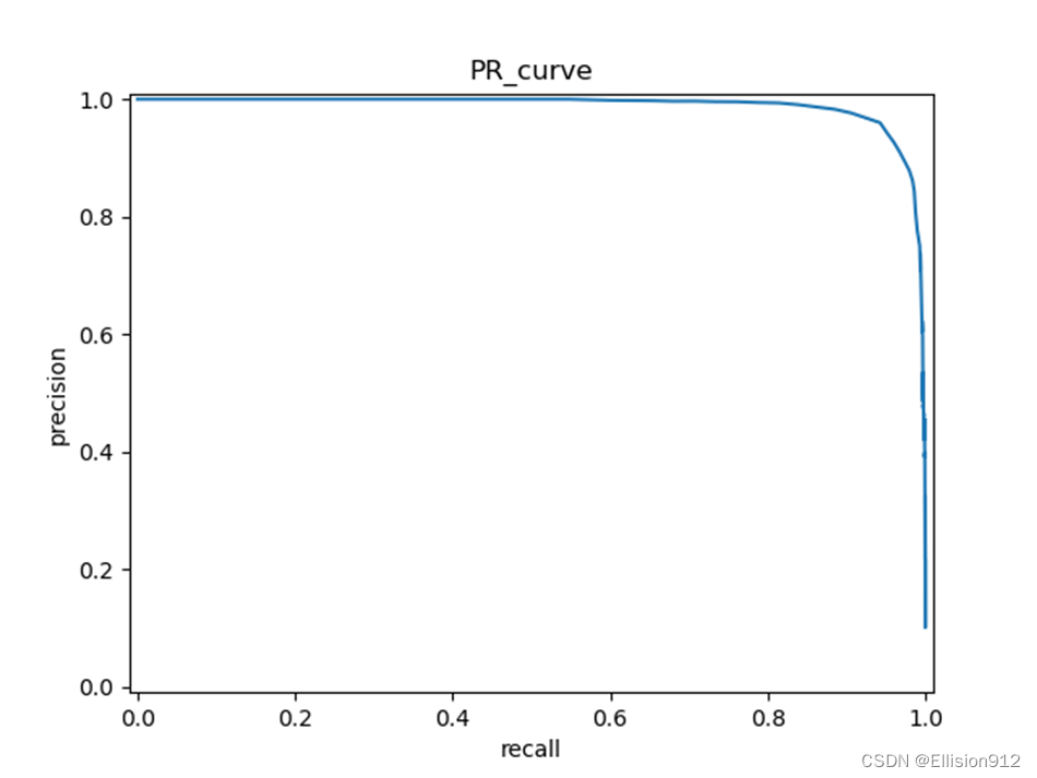
My_net的PR、ROC曲线：

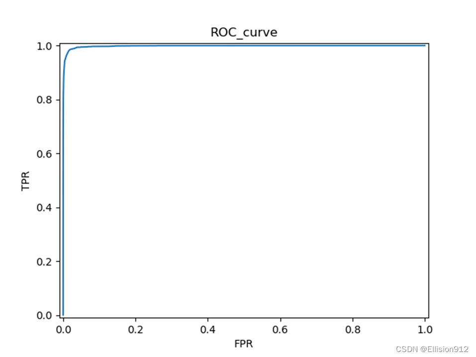
Resnet18的PR、ROC曲线：


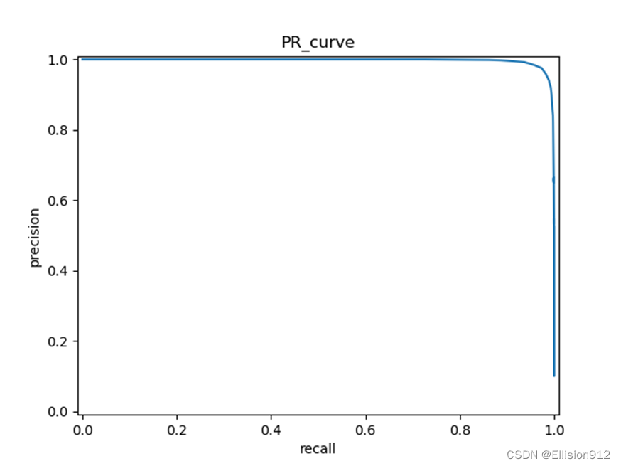
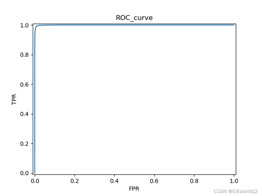
模型简单评估：在同样的学习率、迭代次数下，很明显resnet18的PR曲线和ROC曲线下面积都比My_net的大，说明准确率、精度、查全率更高，从模型精度角度说明resnet18更优，但resnet18有18层网络，而My_net只有2层， My_net更快更小。

下面我贴出可以适用任何简单的分类数据集的数据加载、训练、测试代码，实质上就是本次实验所有的代码和数据，在百度网盘中，下载到本地改一下文件目录就可以运行，尽量没有使用框架。
链接：https://pan.baidu.com/s/1YWbi6a3SM45qrF7W7J1Kog?pwd=nafw
提取码：nafw
有不足之处希望指出我会改正，如果有其他需求可以评论区提问！欢迎点赞收藏！