数字信号处理实验---FFT分析

一、题目：

二、实验要求：

1、绘制图形时，尽量选用已经提供的函数。

2、所有的图形，需要加上横坐标、纵坐标以及标题的说明。

3、将设计的程序保存为脚本文件，在实验报告中，需写出程序语句。

4、Matlab程序中，需要为每段语句添加说明，说清每段的任务是什么，其中语句执行功能是什么

三、评分标准：

1. 用FFT计算其幅度频谱和相位频谱准确；（3*8=24）
2. 抽样信号的波形计算正确；（3*6=18）
3. 原连续信号波形和抽样信号所对应的幅度谱计算正确；（3*8=24）
4. 用IFFT计算时间序列正确；（3*8=24）
5. 图形横坐标、纵坐标以及标题的说明清晰；（5）
6. 程序代码注释清晰。（5）

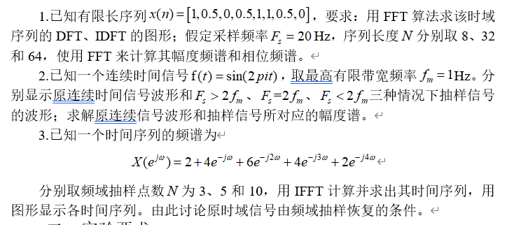
1.% 已知序列

x = [1, 0.5, 0, 0.5, 1, 1, 0.5, 0];

% 计算FFT

X = fft(x);

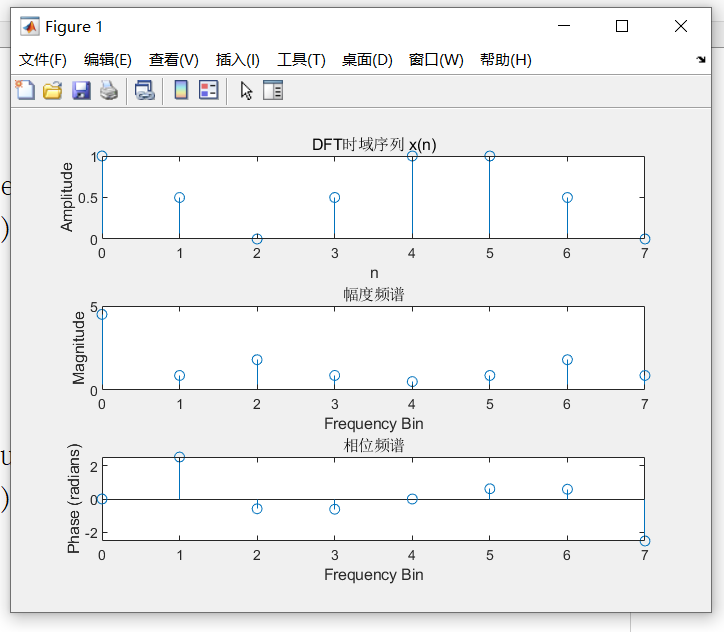
% 计算IDFT

x_reconstructed = ifft(X);

% 时域序列的DFT图形

figure;

subplot(3, 1, 1);

stem(0:length(x)-1, x);

title('DFT时域序列 x(n)');

xlabel('n');

ylabel('Amplitude');

% 幅度频谱图形

subplot(3, 1, 2);

stem(0:length(X)-1, abs(X));

title('幅度频谱');

xlabel('Frequency Bin');

ylabel('Magnitude');

% 相位频谱图形

subplot(3, 1, 3);

stem(0:length(X)-1, angle(X));

title('相位频谱');

xlabel('Frequency Bin');

ylabel('Phase (radians)');

% IDFT图形

figure;

stem(0:length(x_reconstructed)-1, real(x_reconstructed));

title('IDFT 时域序列');

xlabel('n');

ylabel('Amplitude');

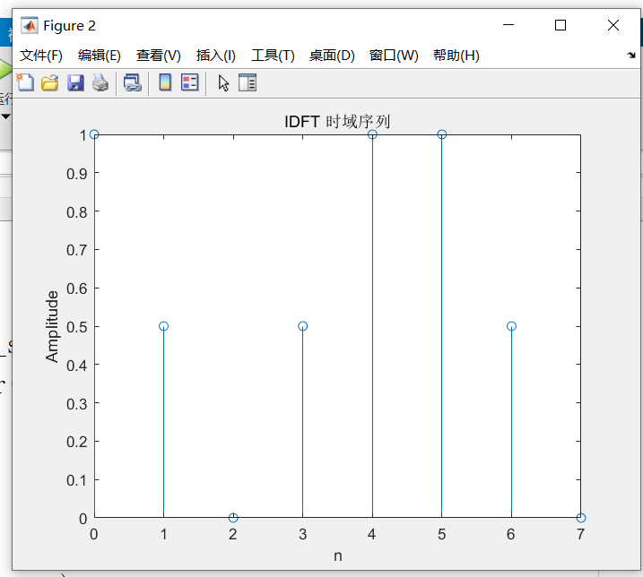
% 已知序列

x = [1, 0.5, 0, 0.5, 1, 1, 0.5, 0];

% 采样频率和序列长度

Fs = 20; % Hz

N_values = [8, 32, 64];

for N = N_values

% 计算FFT

X = fft(x, N);

% 计算幅度谱和相位谱

magnitude_spectrum = abs(X);

phase_spectrum = angle(X);

% 幅度频谱图形

figure;

subplot(2, 1, 1);

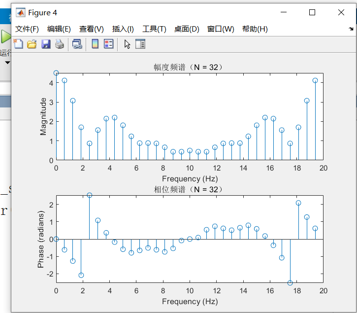
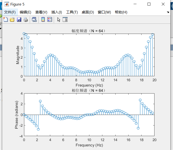
stem((0:N-1)*(Fs/N), magnitude_spectrum);

title(['幅度频谱（N = ' num2str(N) '）']);

xlabel('Frequency (Hz)');

ylabel('Magnitude');

% 相位频谱图形

subplot(2, 1, 2);

stem((0:N-1)*(Fs/N), phase_spectrum);

title(['相位频谱（N = ' num2str(N) '）']);

xlabel('Frequency (Hz)');

ylabel('Phase (radians)');

end

2.% 已知连续时间信号

fm = 1; % Hz，最高有限带宽频率

t_continuous = -1:0.001:1; % 时间范围为 -1 到 1 秒，取足够细的时间步长

f_continuous = sin(2*pi*fm*t_continuous);

% 抽样频率

Fs_values = [2.5*fm, 2*fm, 0.5*fm];

figure;

for i = 1:length(Fs_values)

Fs = Fs_values(i);

Ts = 1/Fs;

% 抽样时间

t_sampled = -1:Ts:1;

% 抽样信号波形

f_sampled = sin(2*pi*fm*t_sampled);

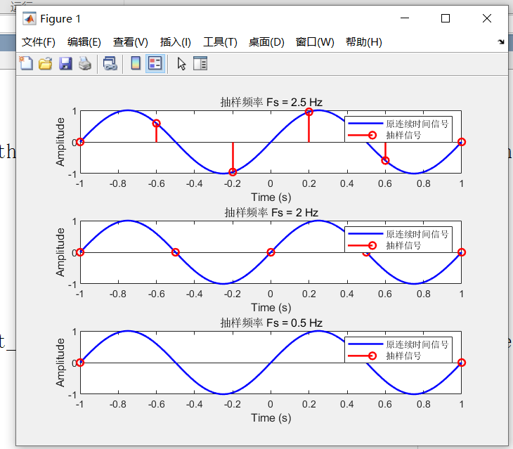
% 绘制原连续时间信号波形

subplot(length(Fs_values), 1, i);

plot(t_continuous, f_continuous, 'b-', 'LineWidth', 1.5);

hold on;

% 绘制抽样信号波形

stem(t_sampled, f_sampled, 'r-', 'LineWidth', 1.5, 'MarkerSize', 6);

title(['抽样频率 Fs = ' num2str(Fs) ' Hz']);

xlabel('Time (s)');

ylabel('Amplitude');

legend('原连续时间信号', '抽样信号');

hold off;

end

% 已知连续时间信号

fm = 1; % Hz，最高有限带宽频率

t_continuous = -1:0.001:1; % 时间范围为 -1 到 1 秒，取足够细的时间步长

f_continuous = sin(2*pi*fm*t_continuous);

% 抽样频率

Fs = 2.5*fm; % 选择一个抽样频率

% 抽样时间

Ts = 1/Fs;

t_sampled = -1:Ts:1;

% 抽样信号波形

f_sampled = sin(2*pi*fm*t_sampled);

% 计算原连续信号的幅度谱

f_continuous_spectrum = abs(fft(f_continuous));

frequencies_continuous = linspace(0, 1/(2*mean(diff(t_continuous))), length(t_continuous)/2);

% 计算抽样信号的幅度谱

f_sampled_spectrum = abs(fft(f_sampled));

frequencies_sampled = linspace(0, Fs, length(t_sampled)/2);

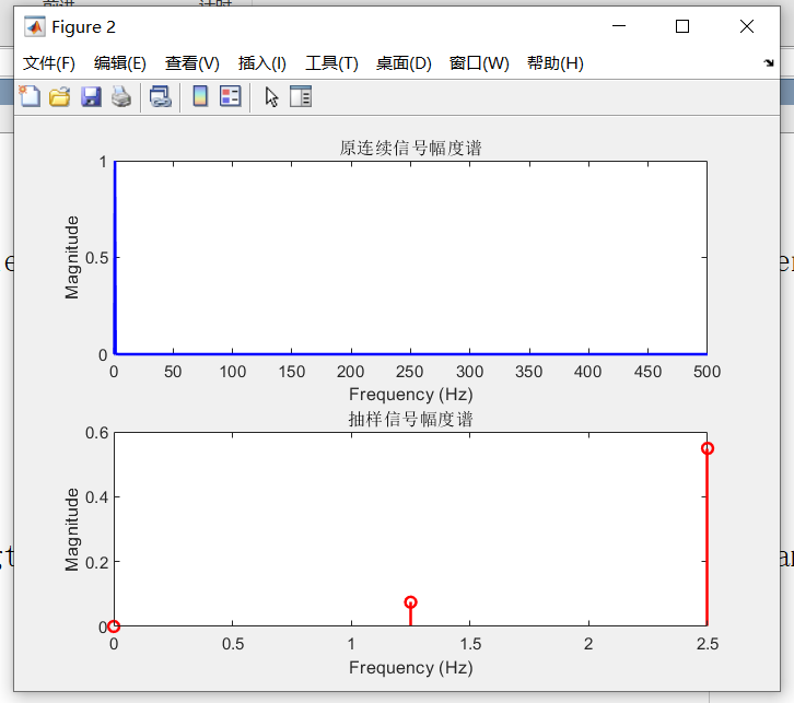
% 绘制原连续信号的幅度谱

figure;

subplot(2, 1, 1);

plot(frequencies_continuous, 2/length(t_continuous) * f_continuous_spectrum(1:length(t_continuous)/2), 'b-', 'LineWidth', 1.5);

title('原连续信号幅度谱');

xlabel('Frequency (Hz)');

ylabel('Magnitude');

% 绘制抽样信号的幅度谱

subplot(2, 1, 2);

stem(frequencies_sampled, 2/length(t_sampled) * f_sampled_spectrum(1:length(t_sampled)/2), 'r-', 'LineWidth', 1.5, 'MarkerSize', 6);

title('抽样信号幅度谱');

xlabel('Frequency (Hz)');

ylabel('Magnitude');

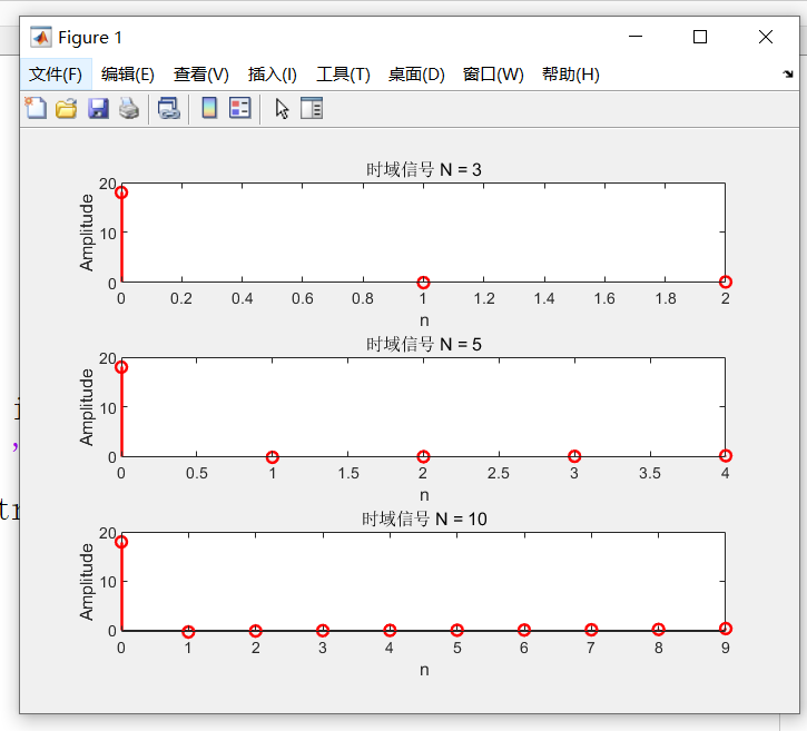
3.% 给定频谱

w = linspace(0, 2*pi, 1000); % 频率范围

X_w = 2 + 4*exp(-1j*w) + 6*exp(-2j*w) + 4*exp(-3j*w) + 2*exp(-4j*w);

% 频域抽样点数

N_values = [3, 5, 10];

figure;

for i = 1:length(N_values)

N = N_values(i);

% 选择前N个频谱样本

X_N = X_w(1:N);

% 使用IFFT计算时域信号

x_n = ifft(X_N, N);

% 绘制时域信号波形

subplot(length(N_values), 1, i);

stem(0:N-1, real(x_n), 'r-', 'LineWidth', 1.5, 'MarkerSize', 6);

title(['时域信号 N = ' num2str(N)]);

xlabel('n');

ylabel('Amplitude');

end