


在Mathematica中内置的绘制Sierpinski地毯的函数:
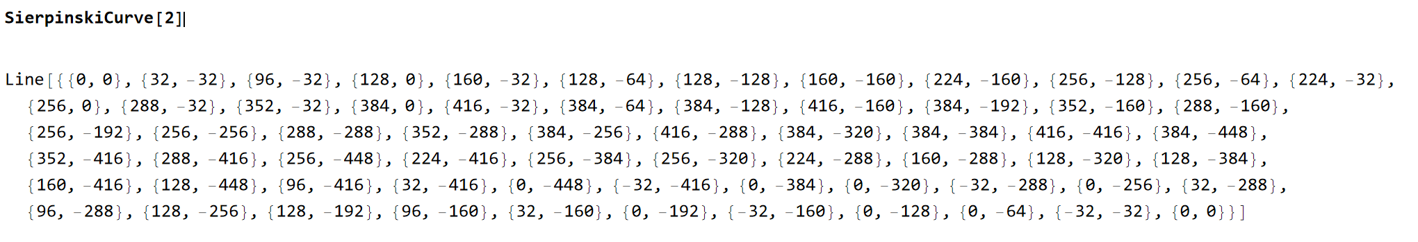
SierpinskiCurve[n]
gives the line segments representing the n-step Sierpiński curve.
注意,直接运行这个函数,返回的是Line对象,例如:
运行如下代码:
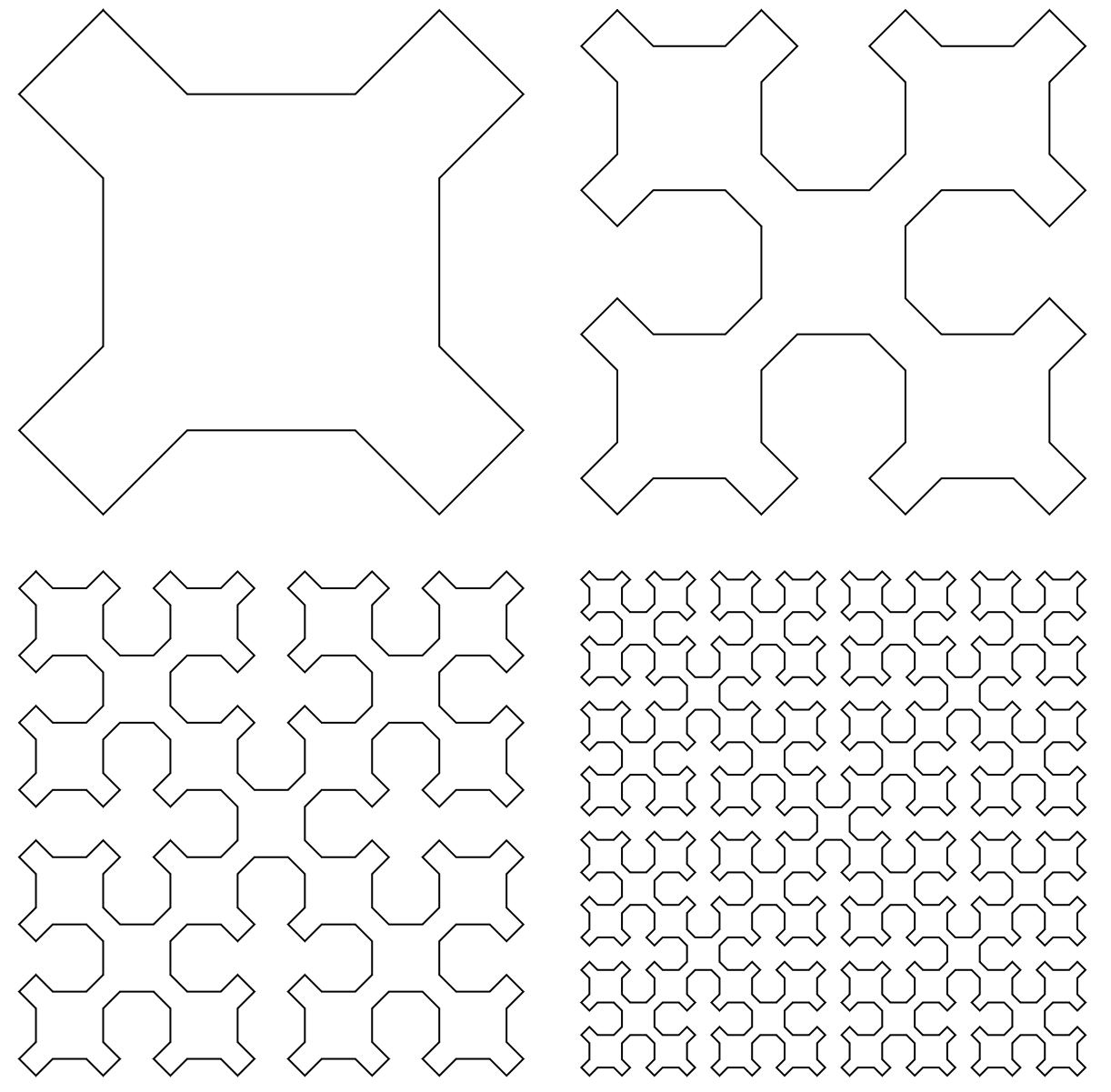
GraphicsGrid[ { {Graphics[SierpinskiCurve[1]], Graphics[SierpinskiCurve[2]]}, {Graphics[SierpinskiCurve[3]], Graphics[SierpinskiCurve[4]]} } ]我们可以得到前面几个地毯的对比图形:
可以通过DataRange,指定参数范围,使得相应的几何图形,能够放在合适的坐标系内:
Graphics[ SierpinskiCurve[3, DataRange -> {{0, 1}, {0, 1}}], PlotRange -> 2, Axes -> True ]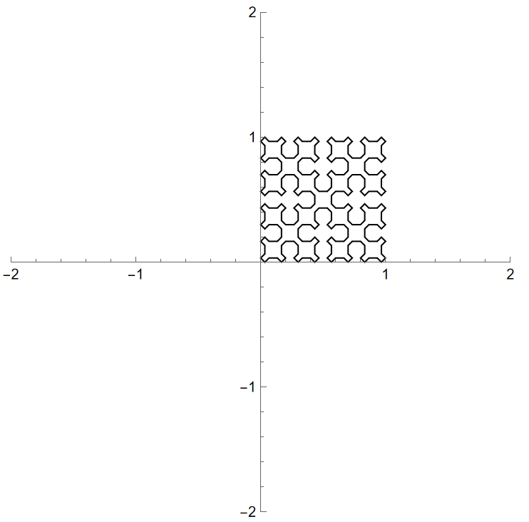
在这个给定的坐标系内,可使用BSplineFunction,将几何图形参数化并绘制出来:
BSplineFunction[ SierpinskiCurve[3, DataRange -> {{-1, 1}, {-1, 1}}][[1]], SplineDegree -> 1]; ParametricPlot[%[t], {t, 0, 1}, PlotPoints -> 400]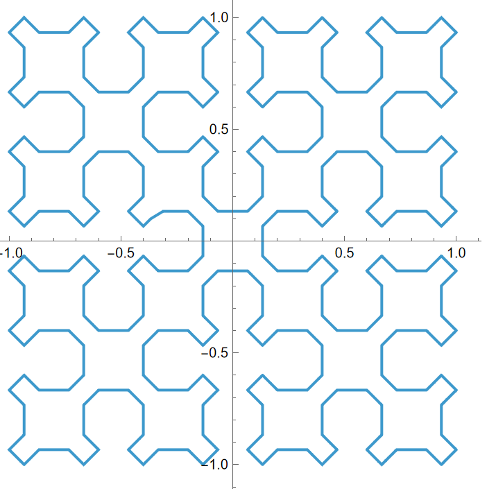
也可以采用如下方式来实现:
Graphics[{Thickness[Large], SierpinskiCurve[3] /. Line -> BSplineCurve}]
注意:此时的BSplineFunction的阶数为2(看起来比上面的要更加光滑)。
利用这个参数化,可以直观看到曲线的填充过程:
tempFunc00 = BSplineFunction[ SierpinskiCurve[4, DataRange -> {{-1, 1}, {-1, 1}}][[1]], SplineDegree -> 1]; Animate[ParametricPlot[tempFunc00[t], {t, 0, n}, PlotPoints -> 400, PlotRange -> {{-1, 1}, {-1, 1}}], {n, 0.01, 1, 0.01}]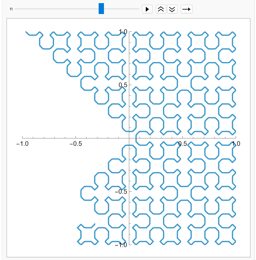
这样的动态效果,是有连续性的视觉效果。但是如果绘制图形的阶数比较大,也可以使用“整数”的方式,来达到类似的视觉效果。
With[{curve = SierpinskiCurve[6]}, Manipulate[ Graphics[{curve, Red, Thick, Line[Take[First[curve], i]]}, ImageSize -> Medium], {i, 1, 16385, 1}]]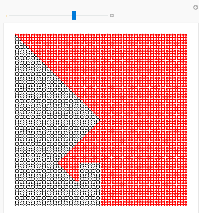


 被折叠的 条评论
为什么被折叠?
被折叠的 条评论
为什么被折叠?
 到【灌水乐园】发言


