Smooth Peter de Jong 奇异吸引子

Smooth Peter de Jong attractor 是混沌理论中的一种奇异吸引子，其动态特性由迭代方程驱动，能够生成复杂且艺术化的分形图案。该吸引子的数学表达式为：

其中，参数 a,b,c,d 的微小变化会显著影响系统的演化轨迹，体现了混沌系统对初值的敏感性（即“蝴蝶效应”）。

特性与行为

1. 混沌与分形：Peter de Jong吸引子的轨迹在二维或三维空间中展开时，会形成非重复的精细结构，具有非整数维度（如2.06维），属于分形几何的典型表现。
2. 参数敏感性：不同参数组合会生成截然不同的图案。例如，a=1.4,b=−2.3,c=2.4,d=−2.1a=1.4,b=−2.3,c=2.4,d=−2.1 会产生密集的螺旋结构，而 a=−0.709,b=1.638a=−0.709,b=1.638 则可能形成对称的星云状图案。
3. 可视化方法：通过迭代计算数百万个点并映射到坐标系中，可生成高分辨率图像。为增强视觉效果，常引入颜色映射（如将第三变量 zz 的迭代结果作为颜色参数），使图像更具层次感。

总结来看，Smooth Peter de Jong attractor 通过简单的非线性方程揭示了复杂系统的内在秩序，成为连接数学、计算机科学与艺术的桥梁。

为了能够看到相应的分形图案，接下来使用Mathematica进行编程绘制。这里以三维空间中来进行示例。

首先，产生相点：

fr2 = Compile[{{p, _Real, 1}, {n, _Integer}, {a, _Real, 1}, {b, _Real,
      1}, {c, _Real, 1}}, 
   NestList[{Sin[a[[1]] #[[2]]] - Cos[a[[2]] #[[1]]], 
      Sin[b[[1]] #[[1]]] - Cos[b[[2]] #[[2]]], 
      Sin[c[[1]] #[[1]]] - Cos[c[[2]] #[[1]]]} &, p, n]];

DynamicModule[{a, b, c, n, type, fig, controls, print}, 
 Deploy@Dynamic[
   Refresh[Panel@Grid[{{fig, controls}}, Spacings -> 2], None]], 
 Initialization :> (type = 1;
   n = 100000;
   {a, b, c} = {{1.4, -2.3}, {2.4, -2.1}, {2.41, 1.64}};
   controls = 
    Column[{Slider2D[Dynamic@a, {-Pi, Pi, .01}], Dynamic@a, 
      Slider2D[Dynamic@b, {-Pi, Pi, .01}], Dynamic@b, 
      Slider2D[Dynamic@c, {-Pi, Pi, .01}], Dynamic@c}];
   fig = 
    Graphics[{White, AbsolutePointSize@1, 
      Dynamic[Point@
        fr2[{.0, .0, .0}, ControlActive[2 10^4, 10^5], a, b, 
          c][[All, ;; 2]]]}, ImageSize -> {1, 1} 500, 
     Background -> Black, AspectRatio -> Automatic];
   print[] := 
    With[{t = 3, pointsize = 1, pts = 10^5, res = 72}, 
     Composition[CreateDocument, 
       ImageResize[Rasterize[#, "Image", ImageResolution -> t res], 
         Scaled[1/t]] &, 
       Graphics[{AbsolutePointSize@pointsize, 
          Riffle[Hue@Rescale[#, {-2, 2}, {0, 1}] & /@ #[[;; , 3]], 
             Point /@ #[[;; , ;; 2]]] &@#}, ImageSize -> 800, 
         Background -> Black] &][fr2[{.0, .0, .0}, pts, a, b, c]]];)]

可以给出一个简单的交互界面：

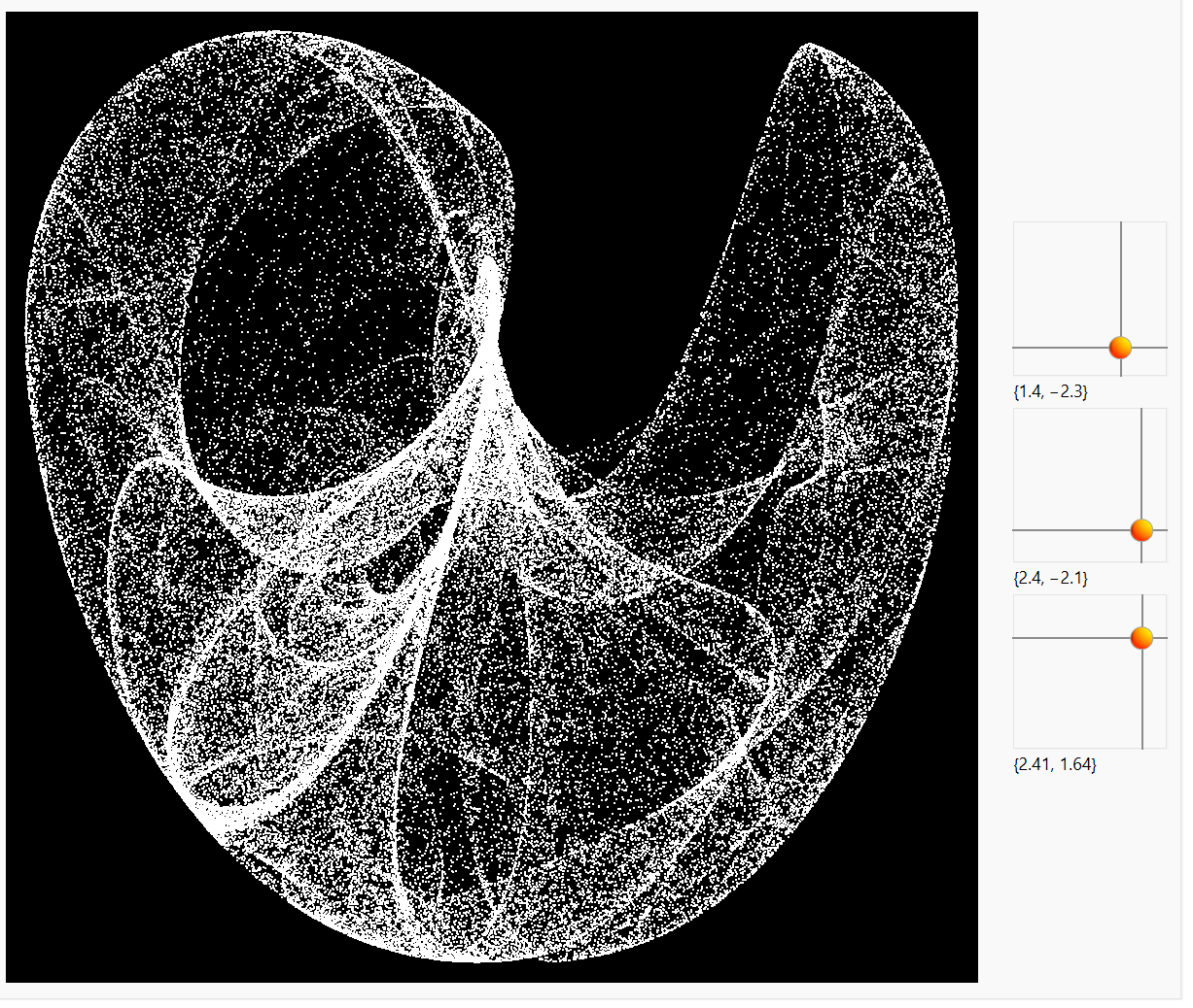
从这个图形中，三个小黄点，分别代表a，b，c的值。通过改变这些参数的值，可以看到不同的图案。将参数c删掉，可以看到二维图案！

在二维情形，可以使用ArrayPlot实现一个简单的彩色绘制：

func = Compile[{{dim, _Integer}, {params, _Real, 1}, {iters, _Integer}},
    Module[{matrix, d1, d2, a, b, c, d, x, y, iter, xp, xn, yp, yn, 
     max}, matrix = Table[0.0, {dim dim}];
    {a, b, c, d, x, y, iter} = params~Join~{0, 0, 1};
    {d1, d2} = {1 + 0.5 (dim - 1), 0.25 (dim - 1)};
    While[++iter < iters, xn = Sin[a y] - Cos[b x]; 
     y = Sin[c x] - Cos[d y]; x = xn;
     xp = Floor[d1 + d2 x]; yp = Floor[d1 - d2 y];
     ++matrix[[yp dim + xp]];];
    max = Max@matrix;
    Partition[(Sqrt[#]/max &) /@ matrix, dim]](*,CompilationTarget->
   "C"*), RuntimeOptions -> "Speed"];

dejong[dim_, params_, iters_] := 
  Module[{matrix}, matrix = func[dim, params, iters];
   Colorize[ArrayPlot[matrix, ImageSize -> dim, Frame -> False], 
    ColorFunction -> ColorData["SunsetColors"]]];
    
dejong[1024, {1.4, -2.3, 2.4, -2.1}, 20000000]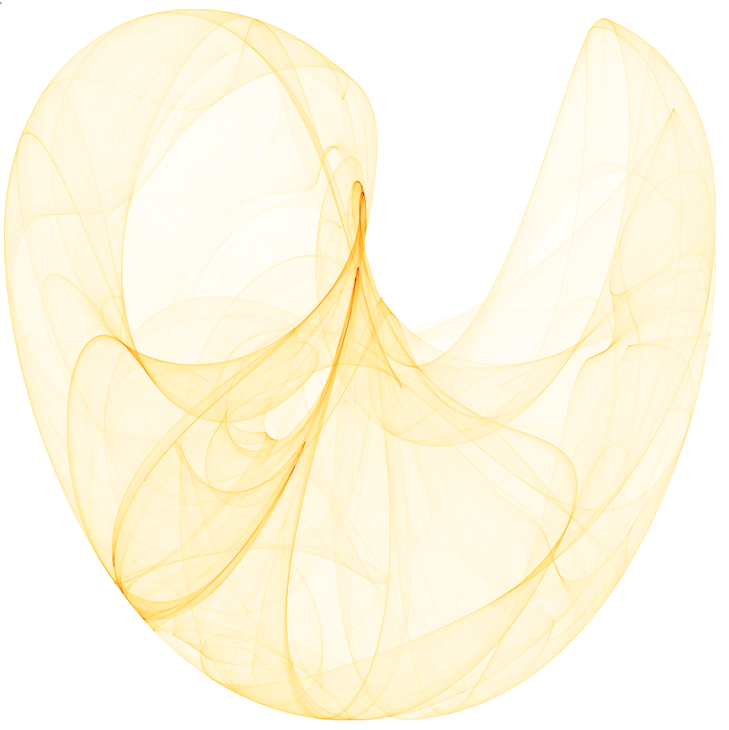

也可以使用级数函数来进行成像：

attractor = 
  Compile[{{xmin, _Real}, {xmax, _Real}, {ymin, _Real}, {ymax, \
_Real}, {delta, _Real}, {itmax, _Integer}, {a, _Real, 1}, {b, _Real, 
     1}}, Block[{bins, d, x, y, tx, ty}, 
    bins = ConstantArray[0, 
      Floor[{xmax - xmin, ymax - ymin}/delta] + {1, 1}];
    d = Dimensions[bins];
    {x, y} = {0., 0.};
    Do[{x, y} = {Sin[a[[1]] y] - Cos[a[[2]] x], 
       Sin[b[[1]] x] - Cos[b[[2]] y]};
     tx = Floor[(x - xmin)/delta] + 1;
     ty = Floor[(y - ymin)/delta] + 1;
     If[tx >= 1 && tx <= d[[1]] && ty >= 1 && ty <= d[[2]], 
      bins[[tx, ty]] += 1], {i, 1, itmax}];
    bins](*,CompilationTarget:>"C"*)];
    
    bins = N[
   attractor[-2., 2., -2.2, 2.2, 0.005, 
    5*10^6, {1.2, -2.1}, {2.4, -2.1}]];
ArrayPlot[Log[bins + 1], 
 ColorFunction -> (ColorData["FallColors", #^0.4] &)]