科技股预测新利器：NLP情绪分析与机器学习的完美融合（三）

本文链接：https://blog.csdn.net/weixin_70955880/article/details/144758098

作者：老余捞鱼

原创不易，转载请标明出处及原作者。

写在前面的话：今天我将完成NLP 情感分析与机器学习融合应用于科技股投资这个系列，本文的主要内容是使用GRU进行股票价格预测，以及使用 MLBC 进行市场情绪分析，这将进一步提升预测的准确性和及时性。

阅读本章节的一些前提：

完成本系列前两章节的学习；
基本掌握了周标量、矢量情绪评分的方法；
熟悉了通过抓取最新的谷歌新闻和使用Yahoo Finance API获取的财务数据；
能对11 种科技股的每日平均矢量情绪得分。

前两个章节的链接如下：

一、GRU 股票价格预测

本章节我们将通过将 NLP 情感分析与 ML 价格预测相结合，获得对科技市场动态的宝贵见解，从而对传统 GRU 分析方法进行补充。

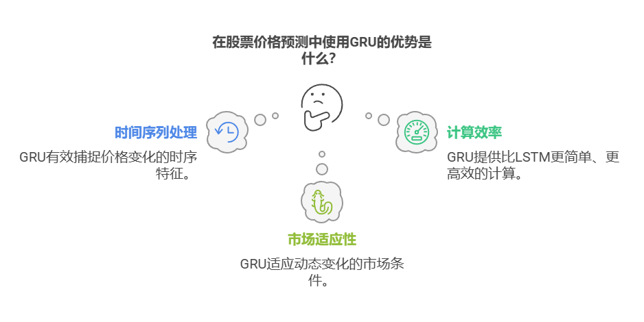
1.1 什么是 GRU？

GRU（门控循环单元）是一种深度学习模型，特别适合处理时间序列数据，如股票价格。通过分析历史数据，GRU能够捕捉价格变化的模式，从而为未来的价格走势提供预测。其基本原理如下图：

GRU是一种改进的循环神经网络（RNN），其设计旨在解决传统RNN在长序列数据处理中的梯度消失问题。GRU通过引入门控机制，能够更有效地选择和更新信息，从而提高模型的学习能力。GRU包含两个主要的门：重置门和更新门，这使得模型能够灵活地决定保留多少过去的信息以及引入多少新的信息。

1.2 如何实现GRU股票价格预测

其实现股票价格预测的流程由以下五步构成：

数据收集：首先，需要收集历史股票价格数据，通常包括开盘价、收盘价、最高价、最低价和成交量等信息。
数据预处理：对数据进行清洗和标准化，以便于模型的训练。
构建模型：使用深度学习框架（如TensorFlow或PyTorch）构建GRU模型，设置适当的超参数。
训练模型：将处理后的数据输入模型进行训练，使用历史数据来优化模型的参数。
预测与评估：使用训练好的模型进行股票价格预测，并通过指标（如均方误差）评估模型的性能。

GRU在股票价格预测中展现出了良好的性能，能够有效捕捉价格变化的时序特征。通过合理的数据处理和模型构建，GRU可以为投资者提供有价值的预测信息，帮助其做出更明智的投资决策。

1.3 具体功能实现

我们还是以 AMZN 股票为例，首先还是导入必要的 Python 库并读取股票数据。

from pyexpat import model
from tabnanny import verbose
import pandas as pd
import numpy as np
import matplotlib.pyplot as plt
import seaborn as sns
#from pandas_datareader import data as pdr
import yfinance as yf
from sklearn.preprocessing import MinMaxScaler
from keras.models import Sequential
from keras.layers import Dense, GRU, Dropout
from datetime import datetime, timedelta



df = yf.download("AMZN", start="2020-01-03", end=datetime.now())

接下来是为 GRU 预测准备缩放的训练集/测试集。

# Create a new dataframe with only the 'Close' column
data = df.filter(['Close'])
# Convert the dataframe to a numpy array
dataset = data.values
# Get the number of rows to train the model on
training_data_len = int(np.ceil(len(dataset) * .95))

train_data = dataset[0:int(training_data_len), :]
test_data = dataset[training_data_len - 60:, :]

# Scale the data
scaler = MinMaxScaler(feature_range=(0, 1))
train_data_sc=scaler.fit_transform(train_data)
test_data_sc=scaler.fit_transform(test_data)

# Split the data into x_train and y_train data sets
x_train = []
y_train = []

for i in range(60, len(train_data_sc)):
    x_train.append(train_data_sc[i-60:i, 0])
    y_train.append(train_data_sc[i, 0])

# Convert the x_train and y_train to numpy arrays 
x_train, y_train = np.array(x_train), np.array(y_train)

# Reshape input data to 3D for GRU [samples, time steps, features]
x_train = np.reshape(x_train, (x_train.shape[0], x_train.shape[1], 1))

利用附加层和剔除构建 GRU 模型。

# Build the GRU model with additional layers and dropout
model = Sequential()

model.add(GRU(units=128, return_sequences=True, input_shape=(x_train.shape[1],1), activation='tanh'))
model.add(Dropout(0.2))

# Second GRU layer
model.add(GRU(units=64, return_sequences=True))
model.add(Dropout(0.2))

# Third GRU layer
model.add(GRU(64,return_sequences=False))
model.add(Dropout(0.2))

# The output layer
model.add(Dense(units=1))

# Compiling the model
model.compile(optimizer='adam',loss='mean_squared_error')

# Fitting to the training set
history =model.fit(x_train,y_train,epochs=50,batch_size=16)

Epoch 1/50
71/71 ━━━━━━━━━━━━━━━━━━━━ 6s 36ms/step - loss: 0.0480
Epoch 2/50
71/71 ━━━━━━━━━━━━━━━━━━━━ 3s 37ms/step - loss: 0.0052
Epoch 3/50
71/71 ━━━━━━━━━━━━━━━━━━━━ 3s 39ms/step - loss: 0.0055
Epoch 4/50
71/71 ━━━━━━━━━━━━━━━━━━━━ 3s 40ms/step - loss: 0.0048
Epoch 5/50
71/71 ━━━━━━━━━━━━━━━━━━━━ 3s 37ms/step - loss: 0.0043
Epoch 6/50
71/71 ━━━━━━━━━━━━━━━━━━━━ 3s 38ms/step - loss: 0.0035
Epoch 7/50
71/71 ━━━━━━━━━━━━━━━━━━━━ 3s 38ms/step - loss: 0.0038
Epoch 8/50
71/71 ━━━━━━━━━━━━━━━━━━━━ 3s 43ms/step - loss: 0.0047
Epoch 9/50
71/71 ━━━━━━━━━━━━━━━━━━━━ 3s 37ms/step - loss: 0.0029
...........................................



print(history.history.keys())

dict_keys(['loss'])

打印 GRU 模式摘要

model.summary()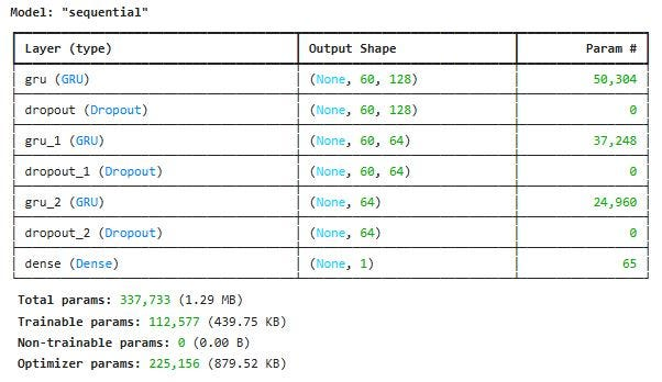

绘制 GRU 损失与时间的关系图

plt.plot(history.history['loss'], label='train')

plt.grid()
plt.legend()
plt.xlabel('Epochs')
plt.ylabel('Loss')
plt.show()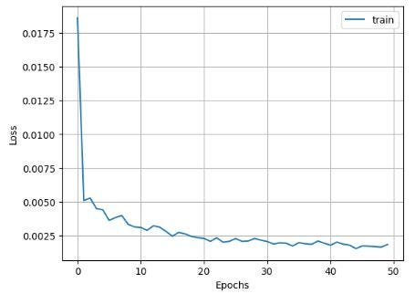

对测试数据进行 GRU 预测

# Create the testing data set
test_data = scaler.fit_transform(dataset[training_data_len - 60:, :])
x_test = []
y_test = scaler.fit_transform(dataset[training_data_len:, :])

for i in range(60, len(test_data)):
    x_test.append(test_data[i-60:i, 0])

# Convert the data to a numpy array
x_test = np.array(x_test)

# Reshape the data
x_test = np.reshape(x_test, (x_test.shape[0], x_test.shape[1], 1))

# Get the model's predicted price values 
predictions = model.predict(x_test)

验证测试预测

# Get the root mean squared error (RMSE)
rmse = np.sqrt(np.mean(((predictions - y_test) ** 2)))
print('RMSE: ', rmse)

RMSE:  0.18898223429208838

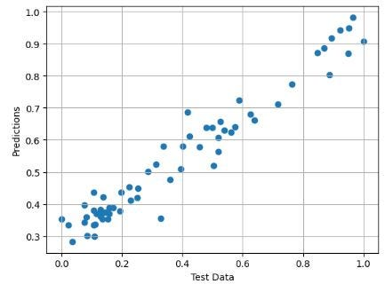
# X-Plot Predictions vs Test Data

plt.scatter(y_test,predictions)
plt.xlabel('Test Data')
plt.ylabel('Predictions')
plt.grid()

得到X-Plot 预测值与测试数据对比图

归一化 AMZN 价格比较 - 预测与测试数据

plt.plot(y_test,label='Test Data')
plt.plot(predictions,label='Predictions')
plt.title('Normalized AMZN Price')
plt.xlabel('Day No')
plt.legend()
plt.grid()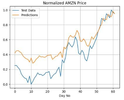

检查 MAE 和 R2 分数

from sklearn.metrics import mean_absolute_error
mean_absolute_error(y_test, predictions)

0.1624050197414233

from sklearn.metrics import r2_score
r2_score(y_test, predictions)

0.5741042876012528

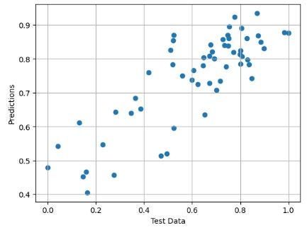
将相同的 GRU 工作流程应用于 NVDA 股价，也能得到类似的结果

print('RMSE: ', rmse)

RMSE:  0.20304139023404796

得到NVDA 股票的 X-Plot 预测与测试数据对比图

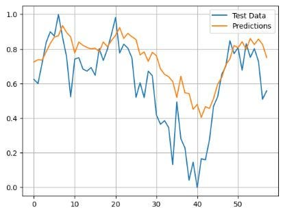
上图为归一化 NVDA 价格 - 预测与测试数据对比图

二、使用 MLBC 进行市场情绪分析与预测

最近的研究表明，MLBC（ ML binary classification）和 NLP 可视化[12]在分析文本情绪方面具有巨大潜力。

本节的目标是解决一个二元分类问题，将道琼斯工业平均指数（DJIA）股票相关情绪数据（新闻标题）分为正面和负面。这里，目标 "标签 "代表以下二元属性：0 - 股价下跌或保持不变，1 - 股价上涨。

步骤 1：导入基本库并读取输入数据集

# Importing essential libraries
import numpy as np
import pandas as pd

# Importing essential libraries for visualization
import matplotlib.pyplot as plt
import seaborn as sns
%matplotlib inline

# Importing essential libraries for performing Natural Language Processing on given dataset
import nltk
nltk.download('stopwords')
from nltk.corpus import stopwords
from nltk.stem import PorterStemmer

# Loading the dataset
df = pd.read_csv('stock_senti_analysis.csv', encoding = 'ISO-8859-1')

df.info()

<class 'pandas.core.frame.DataFrame'>
Index: 4098 entries, 0 to 4100
Data columns (total 27 columns):
 #   Column  Non-Null Count  Dtype 
---  ------  --------------  ----- 
 0   Date    4098 non-null   object
 1   Label   4098 non-null   int64 
 2   Top1    4098 non-null   object
 3   Top2    4098 non-null   object
 4   Top3    4098 non-null   object
 5   Top4    4098 non-null   object
 6   Top5    4098 non-null   object
 7   Top6    4098 non-null   object
 8   Top7    4098 non-null   object
 9   Top8    4098 non-null   object
 10  Top9    4098 non-null   object
 11  Top10   4098 non-null   object
 12  Top11   4098 non-null   object
 13  Top12   4098 non-null   object
 14  Top13   4098 non-null   object
 15  Top14   4098 non-null   object
 16  Top15   4098 non-null   object
 17  Top16   4098 non-null   object
 18  Top17   4098 non-null   object
 19  Top18   4098 non-null   object
 20  Top19   4098 non-null   object
 21  Top20   4098 non-null   object
 22  Top21   4098 non-null   object
 23  Top22   4098 non-null   object
 24  Top23   4098 non-null   object
 25  Top24   4098 non-null   object
 26  Top25   4098 non-null   object
dtypes: int64(1), object(26)
memory usage: 896.4+ KB

df_copy = df.copy()
df_copy.reset_index(inplace=True)

步骤 2：NLP ML 二进制分类的数据预处理

# Splitting the dataset into train an test set
train = df_copy[df_copy['Date'] < '20150101']
test = df_copy[df_copy['Date'] > '20141231']
print('Train size: {}, Test size: {}'.format(train.shape, test.shape))

Train size: (3972, 28), Test size: (378, 28)

# Removing punctuation and special character from the text
train.replace(to_replace='[^a-zA-Z]', value=' ', regex=True, inplace=True)
test.replace(to_replace='[^a-zA-Z]', value=' ', regex=True, inplace=True)

# Renaming columns
new_columns = [str(i) for i in range(0,25)]
train.columns = new_columns
test.columns = new_columns

# Converting the entire text to lower case
for i in new_columns:
  train[i] = train[i].str.lower()
  test[i] = test[i].str.lower()

# Joining all the columns
train_headlines = []
test_headlines = []

for row in range(0, train.shape[0]):
  train_headlines.append(' '.join(str(x) for x in train.iloc[row, 0:25]))

for row in range(0, test.shape[0]):
  test_headlines.append(' '.join(str(x) for x in test.iloc[row, 0:25]))

# Creating corpus of train dataset
ps = PorterStemmer()
train_corpus = []

for i in range(0, len(train_headlines)):
  
  # Tokenizing the news-title by words
  words = train_headlines[i].split()

  # Removing the stopwords
  words = [word for word in words if word not in set(stopwords.words('english'))]

  # Stemming the words
  words = [ps.stem(word) for word in words]

  # Joining the stemmed words
  headline = ' '.join(words)

  # Building a corpus of news-title
  train_corpus.append(headline)

# Creating corpus of test dataset
test_corpus = []

for i in range(0, len(test_headlines)):
  
  # Tokenizing the news-title by words
  words = test_headlines[i].split()

  # Removing the stopwords
  words = [word for word in words if word not in set(stopwords.words('english'))]

  # Stemming the words
  words = [ps.stem(word) for word in words]

  # Joining the stemmed words
  headline = ' '.join(words)

  # Building a corpus of news-title
  test_corpus.append(headline)

步骤 3a：为负面情绪创建词云

down_words = []
for i in list(y_train[y_train==0].index):
  down_words.append(train_corpus[i])

up_words = []
for i in list(y_train[y_train==1].index):
  up_words.append(train_corpus[i])

# Creating wordcloud for down_words
from wordcloud import WordCloud
wordcloud1 = WordCloud(background_color='white', width=3000, height=2500).generate(down_words[1])
plt.figure(figsize=(8,8))
plt.imshow(wordcloud1)
plt.axis('off')
plt.title("Words which indicate a fall in DJIA ")
plt.show()

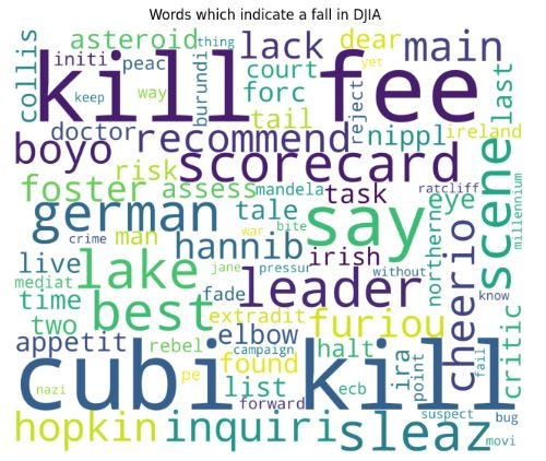
上图为表明道琼斯工业平均指数下跌的词云。

步骤 3b：为正面情绪创建词云

# Creating wordcloud for up_words
wordcloud2 = WordCloud(background_color='white', width=3000, height=2500).generate(up_words[5])
plt.figure(figsize=(8,8))
plt.imshow(wordcloud2)
plt.axis('off')
plt.title("Words which indicate a rise in DJIA ")
plt.show()

上图为表明道琼斯工业平均指数上升的词云。

步骤 4：创建词袋（BOW）模型

# Creating the Bag of Words model
from sklearn.feature_extraction.text import CountVectorizer
cv = CountVectorizer(max_features=10000, ngram_range=(2,2))
X_train = cv.fit_transform(train_corpus).toarray()
X_test = cv.transform(test_corpus).toarray()

步骤 5：训练和验证逻辑回归 (LR)

from sklearn.linear_model import LogisticRegression
lr_classifier = LogisticRegression()
lr_classifier.fit(X_train, y_train)

lr_y_pred = lr_classifier.predict(X_test)

# Accuracy, Precision and Recall
from sklearn.metrics import accuracy_score, precision_score, recall_score
score1 = accuracy_score(y_test, lr_y_pred)
score2 = precision_score(y_test, lr_y_pred)
score3 = recall_score(y_test, lr_y_pred)
print("---- Scores ----")
print("Accuracy score is: {}%".format(round(score1*100,2)))
print("Precision score is: {}".format(round(score2,2)))
print("Recall score is: {}".format(round(score3,2)))

---- Scores ----
Accuracy score is: 85.98%
Precision score is: 0.87
Recall score is: 0.85

# Making the Confusion Matrix
from sklearn.metrics import confusion_matrix
lr_cm = confusion_matrix(y_test, lr_y_pred)

lr_cm

array([[162,  24],
       [ 29, 163]], dtype=int64)

# Plotting the confusion matrix
plt.figure(figsize=(10,7))
sns.heatmap(data=lr_cm, annot=True, cmap="Blues", xticklabels=['Down', 'Up'], yticklabels=['Down', 'Up'])
plt.xlabel('Predicted values')
plt.ylabel('Actual values')
plt.title('Confusion Matrix for Logistic Regression Algorithm')
plt.show()

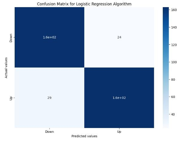
上图为逻辑回归算法的混淆矩阵。

步骤 6：训练和验证随机森林 (RF) 分类器

from sklearn.ensemble import RandomForestClassifier
rf_classifier = RandomForestClassifier(n_estimators=100, criterion='entropy')
rf_classifier.fit(X_train, y_train)

rf_y_pred = rf_classifier.predict(X_test)

# Accuracy, Precision and Recall
score1 = accuracy_score(y_test, rf_y_pred)
score2 = precision_score(y_test, rf_y_pred)
score3 = recall_score(y_test, rf_y_pred)
print("---- Scores ----")
print("Accuracy score is: {}%".format(round(score1*100,2)))
print("Precision score is: {}".format(round(score2,2)))
print("Recall score is: {}".format(round(score3,2)))

---- Scores ----
Accuracy score is: 84.92%
Precision score is: 0.83
Recall score is: 0.88

步骤 7：训练和验证多项式 NB (MNB) 分类器

from sklearn.naive_bayes import MultinomialNB
nb_classifier = MultinomialNB()
nb_classifier.fit(X_train, y_train)

# Predicting the Test set results
nb_y_pred = nb_classifier.predict(X_test)

# Accuracy, Precision and Recall
score1 = accuracy_score(y_test, nb_y_pred)
score2 = precision_score(y_test, nb_y_pred)
score3 = recall_score(y_test, nb_y_pred)
print("---- Scores ----")
print("Accuracy score is: {}%".format(round(score1*100,2)))
print("Precision score is: {}".format(round(score2,2)))
print("Recall score is: {}".format(round(score3,2)))

---- Scores ----
Accuracy score is: 83.86%
Precision score is: 0.85
Recall score is: 0.83

# Making the Confusion Matrix
nb_cm = confusion_matrix(y_test, nb_y_pred)

nb_cm

array([[158,  28],
       [ 33, 159]], dtype=int64)

# Plotting the confusion matrix
plt.figure(figsize=(10,7))
sns.heatmap(data=nb_cm, annot=True, cmap="Blues", xticklabels=['Down', 'Up'], yticklabels=['Down', 'Up'])
plt.xlabel('Predicted values')
plt.ylabel('Actual values')
plt.title('Confusion Matrix for Multinomial Naive Bayes Algorithm')
plt.show()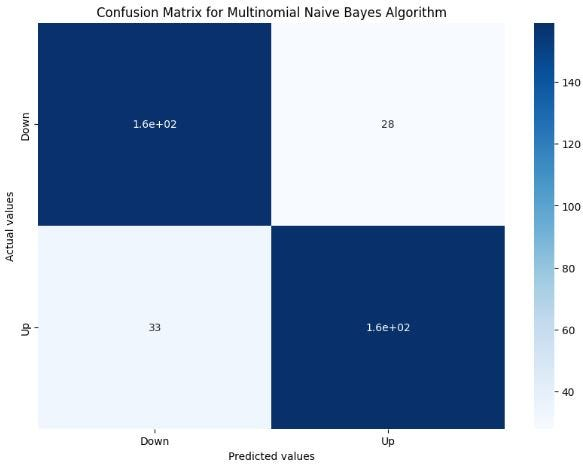

上图为多项式 Naive Bayes 算法的混淆矩阵。

步骤 8：调用 SciKit-Plot ML QC 诊断和 Yellowbrick 可视化（RF示例）

!pip install scikit-plot
!pip install yellowbrick

import scikitplot as skplt

import sklearn

from sklearn.ensemble import RandomForestClassifier, RandomForestRegressor, GradientBoostingClassifier, ExtraTreesClassifier
from sklearn.linear_model import LinearRegression, LogisticRegression

import warnings
warnings.filterwarnings("ignore")

print("Scikit Plot Version : ", skplt.__version__)
print("Scikit Learn Version : ", sklearn.__version__)
print("Python Version : ", sys.version)

%matplotlib inline

Scikit Plot Version :  0.3.7
Scikit Learn Version :  1.4.2
Python Version :  3.12.3 | packaged by conda-forge | (main, Apr 15 2024, 18:20:11) [MSC v.1938 64 bit (AMD64)]

绘制 RF ROC 曲线

Y_test_probs = rf_classifier.predict_proba(X_test)

skplt.metrics.plot_roc_curve(y_test, Y_test_probs,
                       title="RF ROC Curve", figsize=(12,6));
plt.show()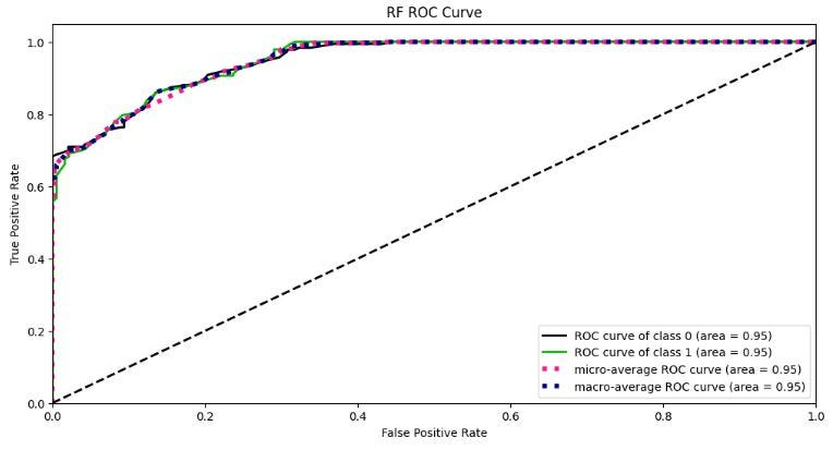

绘制 RF 精度-召回曲线

skplt.metrics.plot_precision_recall_curve(y_test, Y_test_probs,
                       title="RF Precision-Recall Curve", figsize=(12,6));
plt.show()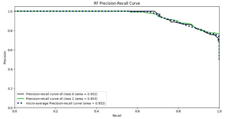

绘制 RF 分类报告

from yellowbrick.classifier import ClassificationReport


target_names=['0','1']

viz = ClassificationReport(RandomForestClassifier(),
                           classes=target_names,
                           support=True,
                           fig=plt.figure(figsize=(12,8)))

viz.fit(X_train, y_train)

viz.score(X_test, y_test)

viz.show();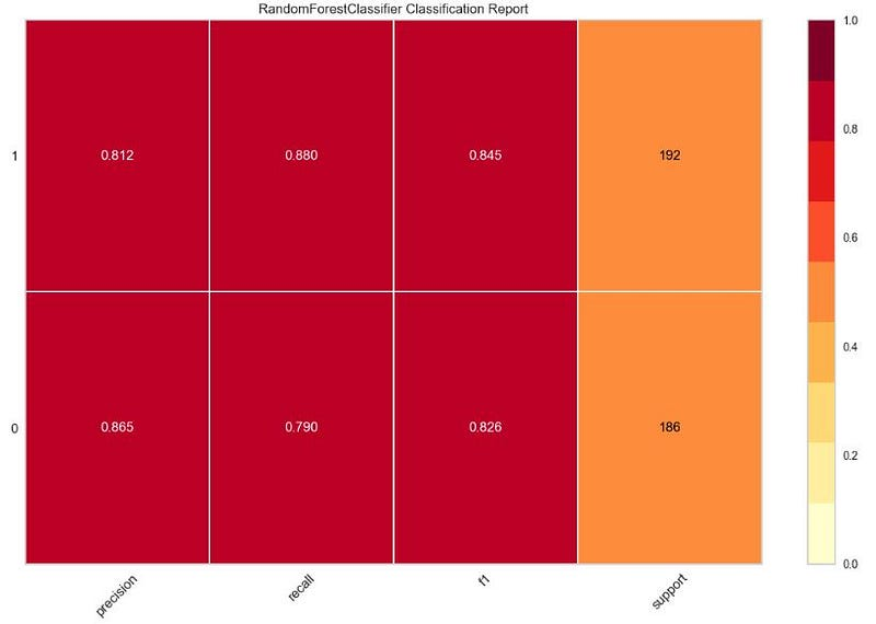

绘制 RF 类别预测误差图

from yellowbrick.classifier import ClassPredictionError

viz = ClassPredictionError(RandomForestClassifier(),
                           classes=target_names,
                           fig=plt.figure(figsize=(9,6)))

viz.fit(X_train, y_train)

viz.score(X_test, y_test)

viz.show();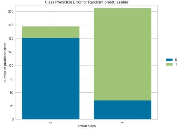

创建 RF KS 统计图

Y_probas = rf_classifier.predict_proba(X_test)

skplt.metrics.plot_ks_statistic(y_test, Y_probas, figsize=(10,6));
plt.show()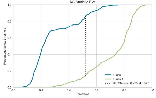

Kolmogorov-Smirnov (KS) 图是统计分析中广泛使用的一种非参数检验，用于比较两种分布。

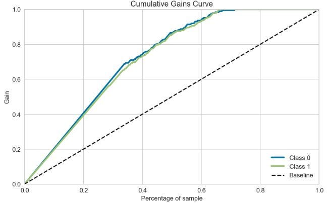
绘制 RF 累积增益曲线

skplt.metrics.plot_cumulative_gain(y_test, Y_probas, figsize=(10,6));
plt.show()

绘制 RF 提升曲线

skplt.metrics.plot_lift_curve(y_test, Y_probas, figsize=(10,6));
plt.show()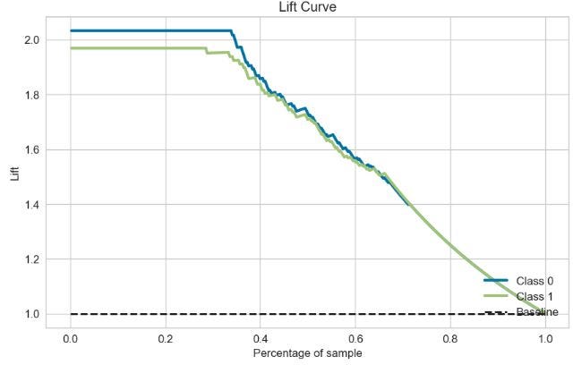

步骤 9：创建和比较 SciKit-Plot 校准曲线

lr_probas = LogisticRegression().fit(X_train, y_train).predict_proba(X_test)
rf_probas = RandomForestClassifier().fit(X_train, y_train).predict_proba(X_test)
gb_probas = GradientBoostingClassifier().fit(X_train, y_train).predict_proba(X_test)
et_scores = ExtraTreesClassifier().fit(X_train, y_train).predict_proba(X_test)

probas_list = [lr_probas, rf_probas, gb_probas, et_scores]
clf_names = ['Logistic Regression', 'Random Forest', 'Gradient Boosting', 'Extra Trees Classifier']

skplt.metrics.plot_calibration_curve(y_test,
                                     probas_list,
                                     clf_names, n_bins=15,
                                     figsize=(12,6)
                                     );
plt.show()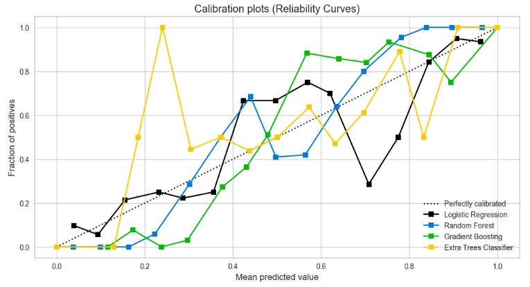

上图为SciKit-Plot 校准曲线图。

关键可视化说明

plt 散点图：每周复合得分与正得分（符号大小）和负得分（符号颜色）的比较。
NLP 向量情绪得分与投资组合中股票总价值（美元）的柱状图。
Plotly 中的互动式股票情绪树状图。
归一化股票价格 - ML 预测与测试数据对比。
制作正面/负面单词的词云。
二元分类器的混淆矩阵、分类报告、ROC、精度-召回、KS 统计量、累积增益、提升、校准曲线和类别预测误差柱状图。

ML/DL 验证结果

用于（归一化）股价预测的 GRU 模型：RMSE (AMZN) ~ 0.19, RMSE (NVDA) ~ 0.2
NLP 和有监督的 ML 二进制分类：

LR
----------------------
Accuracy score is: 85.98%
Precision score is: 0.87
Recall score is: 0.85

RF
----------------------
Accuracy score is: 84.92%
Precision score is: 0.83
Recall score is: 0.88

MNB
----------------------
Accuracy score is: 83.86%
Precision score is: 0.85
Recall score is: 0.83

深入了解 SciKit-Plot ML QC 诊断和 Yellowbrick 可视化（RF示例）：

2 个等级的 ROC 和精确度 - 召回区域：0.95；
KS 统计图：0.520 时为 0.725。
分类报告：F1 分数 ~ 0.8。
预测类别数的类别预测误差 ~ 25。
两个累积增益和提升曲线与基准线相差很大。
当平均预测值超过 90% 时，LR、RF、GB 和 ET 分类器的校准曲线也呈现出类似的趋势。

三、观点总结

本文介绍了一个完全可用的 NLP ML 平台，用于预测（科技）股票数据，并通过分析财经新闻头条来计算标量或矢量情感分数。NLP情感分析作为关键创新点，运用单词嵌入与矢量化技术，能够从经过解析和标注的实时文本数据中提取情感信息。此外，我们所采用的混合方法综合了有监督的机器学习/深度学习算法、自然语言处理以及金融分析技术，充分展示了其在辅助投资者进行决策方面的巨大潜力。

实施 NLP 分析 (VADER)，从每周标量/矢量情感得分的角度研究科技股头条新闻。
观察到 AMZN 每周价格变化与来自finviz.com的情绪评分之间存在适度相关性。
从抓取的近期谷歌新闻中提取的 AMZN 矢量情感评分。
比较了 11 种科技股的每日平均矢量情绪得分。这一附加信息有助于更准确地预测市场趋势。
利用 NLP 情绪分析做出明智的投资决策。我们可以将投资组合中的股票总价值与 4 个平均情绪得分进行比较。但关键是使用 Plotly 创建交互式股票情绪树状图。
实施了一个简单的深度学习（GRU）模型，用于预测股票价格。这样，我们就能获得对科技市场动态的宝贵见解，与 NLP 情绪分析相辅相成。
利用监督 ML 解决二元分类问题，将道琼斯工业平均指数（DJIA）股票相关情绪数据（新闻标题）分为正面和负面。

感谢您阅读到最后，希望本文能给您带来新的收获。码字不易，请帮我点赞、分享。祝您投资顺利！如果对文中的内容有任何疑问，请给我留言，必复。

本文内容仅限技术探讨和学习，不构成任何投资建议