NNDL 作业8：RNN - 简单循环网络

简单循环网络 （ Simple Recurrent Network ， SRN） 只有一个隐藏层的神经网络 ．

目录

1. 使用Numpy实现SRN

 2. 在1的基础上，增加激活函数tanh

 3. 分别使用nn.RNNCell、nn.RNN实现SRN

 4. 分析“二进制加法” 源代码（选做）

5. 实现“Character-Level Language Models”源代码（必做）

6. 分析“序列到序列”源代码（选做）

7. “编码器-解码器”的简单实现（必做）

---

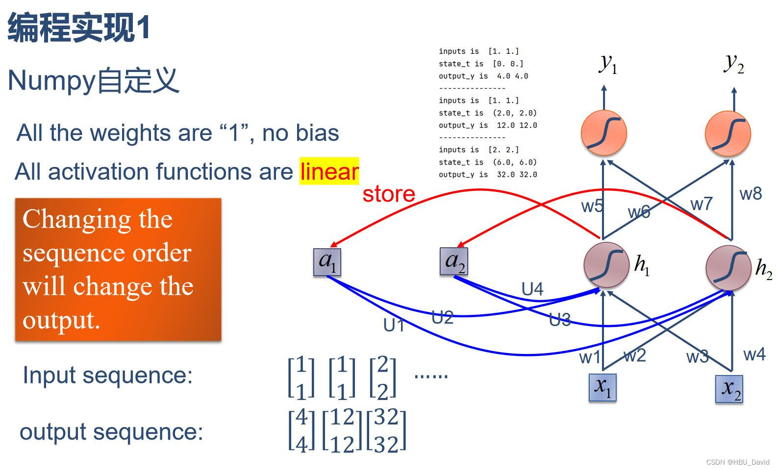
1. 使用Numpy实现SRN

import numpy as np

inputs = np.array([[1., 1.],
                   [1., 1.],
                   [2., 2.]])  # 初始化输入序列
print('inputs is ', inputs)

state_t = np.zeros(2, )  # 初始化存储器
print('state_t is ', state_t)

w1, w2, w3, w4, w5, w6, w7, w8 = 1., 1., 1., 1., 1., 1., 1., 1.
U1, U2, U3, U4 = 1., 1., 1., 1.
print('--------------------------------------')
for input_t in inputs:
    print('inputs is ', input_t)
    print('state_t is ', state_t)
    in_h1 = np.dot([w1, w3], input_t) + np.dot([U2, U4], state_t)
    in_h2 = np.dot([w2, w4], input_t) + np.dot([U1, U3], state_t)
    state_t = in_h1, in_h2
    output_y1 = np.dot([w5, w7], [in_h1, in_h2])
    output_y2 = np.dot([w6, w8], [in_h1, in_h2])
    print('output_y is ', output_y1, output_y2)
    print('---------------')

 2. 在1的基础上，增加激活函数tanh

import numpy as np
 
inputs = np.array([[1., 1.],
                   [1., 1.],
                   [2., 2.]])  # 初始化输入序列
print('inputs is ', inputs)
 
state_t = np.zeros(2, )  # 初始化存储器
print('state_t is ', state_t)
 
w1, w2, w3, w4, w5, w6, w7, w8 = 1., 1., 1., 1., 1., 1., 1., 1.
U1, U2, U3, U4 = 1., 1., 1., 1.
print('--------------------------------------')
for input_t in inputs:
    print('inputs is ', input_t)
    print('state_t is ', state_t)
    in_h1 = np.tanh(np.dot([w1, w3], input_t) + np.dot([U2, U4], state_t))
    in_h2 = np.tanh(np.dot([w2, w4], input_t) + np.dot([U1, U3], state_t))
    state_t = in_h1, in_h2
    output_y1 = np.dot([w5, w7], [in_h1, in_h2])
    output_y2 = np.dot([w6, w8], [in_h1, in_h2])
    print('output_y is ', output_y1, output_y2)
    print('---------------')

 3. 分别使用nn.RNNCell、nn.RNN实现SRN

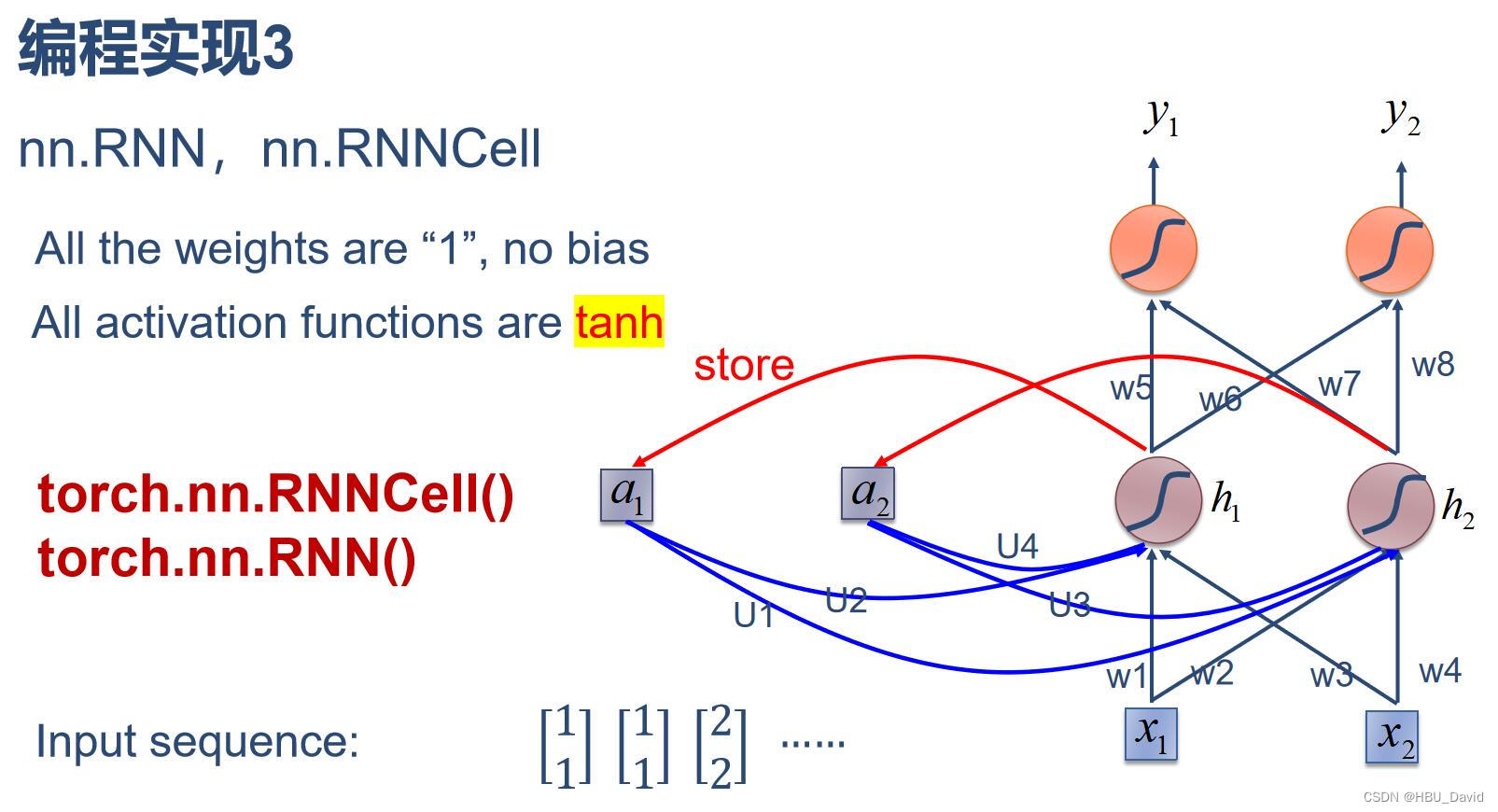
nn.RNNCell:

import torch
 
batch_size = 1
seq_len = 3  # 序列长度
input_size = 2  # 输入序列维度
hidden_size = 2  # 隐藏层维度
output_size = 2  # 输出层维度
 
# RNNCell
cell = torch.nn.RNNCell(input_size=input_size, hidden_size=hidden_size)
# 初始化参数 https://zhuanlan.zhihu.com/p/342012463
for name, param in cell.named_parameters():
    if name.startswith("weight"):
        torch.nn.init.ones_(param)
    else:
        torch.nn.init.zeros_(param)
# 线性层
liner = torch.nn.Linear(hidden_size, output_size)
liner.weight.data = torch.Tensor([[1, 1], [1, 1]])
liner.bias.data = torch.Tensor([0.0])
 
seq = torch.Tensor([[[1, 1]],
                    [[1, 1]],
                    [[2, 2]]])
hidden = torch.zeros(batch_size, hidden_size)
output = torch.zeros(batch_size, output_size)
 
for idx, input in enumerate(seq):
    print('=' * 20, idx, '=' * 20)
 
    print('Input :', input)
    print('hidden :', hidden)
 
    hidden = cell(input, hidden)
    output = liner(hidden)
    print('output :', output)

 nn.RNN:

import torch
 
batch_size = 1
seq_len = 3
input_size = 2
hidden_size = 2
num_layers = 1
output_size = 2
 
cell = torch.nn.RNN(input_size=input_size, hidden_size=hidden_size, num_layers=num_layers)
for name, param in cell.named_parameters():  # 初始化参数
    if name.startswith("weight"):
        torch.nn.init.ones_(param)
    else:
        torch.nn.init.zeros_(param)
 
# 线性层
liner = torch.nn.Linear(hidden_size, output_size)
liner.weight.data = torch.Tensor([[1, 1], [1, 1]])
liner.bias.data = torch.Tensor([0.0])
 
inputs = torch.Tensor([[[1, 1]],
                       [[1, 1]],
                       [[2, 2]]])
hidden = torch.zeros(num_layers, batch_size, hidden_size)
out, hidden = cell(inputs, hidden)
 
print('Input :', inputs[0])
print('hidden:', 0, 0)
print('Output:', liner(out[0]))
print('--------------------------------------')
print('Input :', inputs[1])
print('hidden:', out[0])
print('Output:', liner(out[1]))
print('--------------------------------------')
print('Input :', inputs[2])
print('hidden:', out[1])
print('Output:', liner(out[2]))

  

对比：

torch.RNN()调用的是循环神经网络最原始的形态，这种没法处理比较长的时间序列。最后训练结束，就是最后一个时刻模型所有神经元的输出。对比的是RNNCell区别就是，RNN是读取了0时刻的隐层信息h0，剩下的过程是自动循环完成的，而RNNCell就需要自己写循环处理了

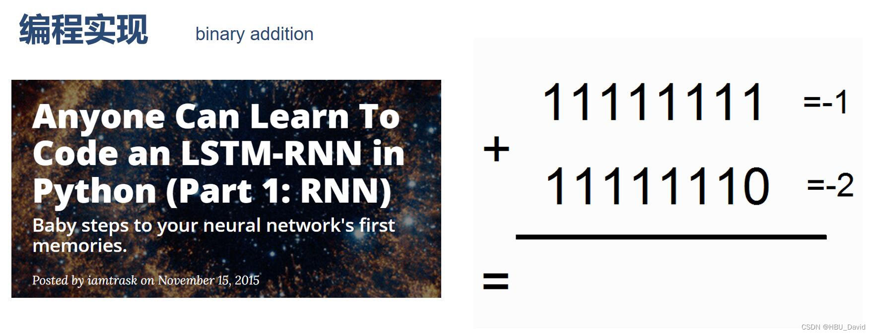
 4. 分析“二进制加法” 源代码（选做）

 

import copy, numpy as np
np.random.seed(0)
 
 
# compute sigmoid nonlinearity
def sigmoid(x):
    output = 1 / (1 + np.exp(-x))
    return output
 
 
# convert output of sigmoid function to its derivative
def sigmoid_output_to_derivative(output):
    return output * (1 - output)
 
 
# training dataset generation
int2binary = {}
binary_dim = 8
 
largest_number = pow(2, binary_dim)
binary = np.unpackbits(
    np.array([range(largest_number)], dtype=np.uint8).T, axis=1)
for i in range(largest_number):
    int2binary[i] = binary[i]
 
# input variables
alpha = 0.1
input_dim = 2
hidden_dim = 16
output_dim = 1
 
# initialize neural network weights
synapse_0 = 2 * np.random.random((input_dim, hidden_dim)) - 1
synapse_1 = 2 * np.random.random((hidden_dim, output_dim)) - 1
synapse_h = 2 * np.random.random((hidden_dim, hidden_dim)) - 1
 
synapse_0_update = np.zeros_like(synapse_0)
synapse_1_update = np.zeros_like(synapse_1)
synapse_h_update = np.zeros_like(synapse_h)
 
# training logic
for j in range(10000):
 
    # generate a simple addition problem (a + b = c)
    a_int = np.random.randint(largest_number / 2)  # int version
    a = int2binary[a_int]  # binary encoding
 
    b_int = np.random.randint(largest_number / 2)  # int version
    b = int2binary[b_int]  # binary encoding
 
    # true answer
    c_int = a_int + b_int
    c = int2binary[c_int]
 
    # where we'll store our best guess (binary encoded)
    d = np.zeros_like(c)
 
    overallError = 0
 
    layer_2_deltas = list()
    layer_1_values = list()
    layer_1_values.append(np.zeros(hidden_dim))
 
    # moving along the positions in the binary encoding
    for position in range(binary_dim):
        # generate input and output
        X = np.array([[a[binary_dim - position - 1], b[binary_dim - position - 1]]])
        y = np.array([[c[binary_dim - position - 1]]]).T
 
        # hidden layer (input ~+ prev_hidden)
        layer_1 = sigmoid(np.dot(X, synapse_0) + np.dot(layer_1_values[-1], synapse_h))
 
        # output layer (new binary representation)
        layer_2 = sigmoid(np.dot(layer_1, synapse_1))
 
        # did we miss?... if so, by how much?
        layer_2_error = y - layer_2
        layer_2_deltas.append((layer_2_error) * sigmoid_output_to_derivative(layer_2))
        overallError += np.abs(layer_2_error[0])
 
        # decode estimate so we can print it out
        d[binary_dim - position - 1] = np.round(layer_2[0][0])
 
        # store hidden layer so we can use it in the next timestep
        layer_1_values.append(copy.deepcopy(layer_1))
 
    future_layer_1_delta = np.zeros(hidden_dim)
 
    for position in range(binary_dim):
        X = np.array([[a[position], b[position]]])
        layer_1 = layer_1_values[-position - 1]
        prev_layer_1 = layer_1_values[-position - 2]
 
        # error at output layer
        layer_2_delta = layer_2_deltas[-position - 1]
        # error at hidden layer
        layer_1_delta = (future_layer_1_delta.dot(synapse_h.T) + layer_2_delta.dot(
            synapse_1.T)) * sigmoid_output_to_derivative(layer_1)
 
        # let's update all our weights so we can try again
        synapse_1_update += np.atleast_2d(layer_1).T.dot(layer_2_delta)
        synapse_h_update += np.atleast_2d(prev_layer_1).T.dot(layer_1_delta)
        synapse_0_update += X.T.dot(layer_1_delta)
 
        future_layer_1_delta = layer_1_delta
 
    synapse_0 += synapse_0_update * alpha
    synapse_1 += synapse_1_update * alpha
    synapse_h += synapse_h_update * alpha
 
    synapse_0_update *= 0
    synapse_1_update *= 0
    synapse_h_update *= 0
 
    # print out progress
    if (j % 1000 == 0):
        print
        "Error:" + str(overallError)
        print("Pred:" + str(d))
        print("True:" + str(c))
        out = 0
        for index, x in enumerate(reversed(d)):
            out += x * pow(2, index)
        print(str(a_int) + " + " + str(b_int) + " = " + str(out))
        print("------------")

Pred:[0 0 0 0 0 0 0 1]
True:[0 1 0 0 0 1 0 1]
9 + 60 = 1
------------
Pred:[1 1 1 1 1 1 1 1]
True:[0 0 1 1 1 1 1 1]
28 + 35 = 255
------------
Pred:[0 1 0 0 1 0 0 0]
True:[1 0 1 0 0 0 0 0]
116 + 44 = 72
------------
Pred:[1 1 0 1 1 1 1 1]
True:[0 1 0 0 1 1 0 1]
4 + 73 = 223
------------
Pred:[0 0 0 0 1 0 0 0]
True:[0 1 0 1 0 0 1 0]
71 + 11 = 8
------------
Pred:[1 0 1 0 0 0 1 0]
True:[1 1 0 0 0 0 1 0]
81 + 113 = 162
------------
Pred:[0 1 0 1 0 0 0 1]
True:[0 1 0 1 0 0 0 1]
81 + 0 = 81
------------
Pred:[1 0 0 0 0 0 0 1]
True:[1 0 0 0 0 0 0 1]
4 + 125 = 129
------------
Pred:[0 0 1 1 1 0 0 0]
True:[0 0 1 1 1 0 0 0]
39 + 17 = 56
------------
Pred:[0 0 0 0 1 1 1 0]
True:[0 0 0 0 1 1 1 0]
11 + 3 = 14
------------

Process finished with exit code 0

1.先定义sigmoid和sigmoid导数函数。
2.初始化8位二进制序列的编码，0-256分别对应00000000-11111111的编码序列。
3.随机产生网络权重，设置随机种子保证每次产生的权重相同，
4.每次训练我们在0-128中随机产生两个数（不是0-256防止溢出），找到对应的8位二进制序列，进行数据输入。
5.开始训练，每1000次查看一次中间结果，产生的结果和正确的结果进行误差计算，从而更新随机网络权重的参数，再次训练再更新，直至我们训练10000次为止（或者可以设置误差小于多少停止）

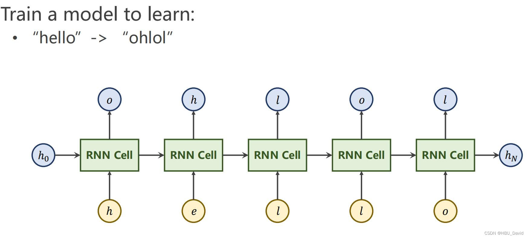
5. 实现“Character-Level Language Models”源代码（必做）

  翻译Character-Level Language Models 相关内容

The Unreasonable Effectiveness of Recurrent Neural Networks

 

As a working example, suppose we only had a vocabulary of four possible letters “helo”, and wanted to train an RNN on the training sequence “hello”. This training sequence is in fact a source of 4 separate training examples: 1. The probability of “e” should be likely given the context of “h”, 2. “l” should be likely in the context of “he”, 3. “l” should also be likely given the context of “hel”, and finally 4. “o” should be likely given the context of “hell”.

Concretely, we will encode each character into a vector using 1-of-k encoding (i.e. all zero except for a single one at the index of the character in the vocabulary), and feed them into the RNN one at a time with the step function. We will then observe a sequence of 4-dimensional output vectors (one dimension per character), which we interpret as the confidence the RNN currently assigns to each character coming next in the sequence. Here’s a diagram:

For example, we see that in the first time step when the RNN saw the character “h” it assigned confidence of 1.0 to the next letter being “h”, 2.2 to letter “e”, -3.0 to “l”, and 4.1 to “o”. Since in our training data (the string “hello”) the next correct character is “e”, we would like to increase its confidence (green) and decrease the confidence of all other letters (red). Similarly, we have a desired target character at every one of the 4 time steps that we’d like the network to assign a greater confidence to. Since the RNN consists entirely of differentiable operations we can run the backpropagation algorithm (this is just a recursive application of the chain rule from calculus) to figure out in what direction we should adjust every one of its weights to increase the scores of the correct targets (green bold numbers). We can then perform a parameter update, which nudges every weight a tiny amount in this gradient direction. If we were to feed the same inputs to the RNN after the parameter update we would find that the scores of the correct characters (e.g. “e” in the first time step) would be slightly higher (e.g. 2.3 instead of 2.2), and the scores of incorrect characters would be slightly lower. We then repeat this process over and over many times until the network converges and its predictions are eventually consistent with the training data in that correct characters are always predicted next.

作为一个工作示例，假设我们只有四个可能的字母“helo”的词汇表，并且想在训练序列“hello”上训练一个RNN。这个训练序列实际上是 4 个独立训练示例的来源：1. 给定 “h” 上下文时，“e”的概率应该可能，2. “l”应该在“he”的上下文中出现，3. “l”也应该在给定“hel”的上下文中，最后是 4。“o”应该可能被赋予“地狱”的上下文。

具体来说，我们将使用 1-of-k 编码将每个字符编码到一个向量中（即除了词汇表中字符索引处的单个字符之外的所有字符均为零），并使用函数一次将它们馈送到 RNN 中。然后，我们将观察一个 4 维输出向量序列（每个字符一个维度），我们将其解释为 RNN 当前分配给序列中下一个字符的置信度。

例如，我们看到，在第一个时间步中，当 RNN 看到字符 “h” 时，它为下一个字母 “h” 分配了 1.0 的置信度，为字母 “e” 分配了 2.2，为 “l” 分配了 -3.0，为 “o” 分配了 4.1 的置信度。由于在我们的训练数据（字符串“hello”）中，下一个正确的字符是“e”，我们希望增加它的置信度（绿色）并降低所有其他字母（红色）的置信度。同样，我们在 4 个时间步中的每一个都有一个期望的目标字符，我们希望网络为其分配更大的置信度。由于 RNN 完全由可微运算组成，我们可以运行反向传播算法（这只是微积分中链式规则的递归应用）来弄清楚我们应该在哪个方向调整其每个权重以增加正确目标的分数（绿色粗体数字）。然后，我们可以执行参数更新，在这个梯度方向上稍微推动每个权重。如果我们在参数更新后将相同的输入提供给 RNN，我们会发现正确字符的分数（例如第一个时间步中的“e”）会略高（例如 2.3 而不是 2.2），而不正确字符的分数会略低。然后，我们一遍又一遍地重复这个过程，直到网络收敛，并且它的预测最终与训练数据一致，因为接下来总是预测正确的字符。

编码实现该模型  

import torch
 
# 使用RNN 有嵌入层和线性层
num_class = 4  # 4个类别
input_size = 4  # 输入维度是4
hidden_size = 8  # 隐层是8个维度
embedding_size = 10  # 嵌入到10维空间
batch_size = 1
num_layers = 2  # 两层的RNN
seq_len = 5  # 序列长度是5
 
# 准备数据
idx2char = ['e', 'h', 'l', 'o']  # 字典
x_data = [[1, 0, 2, 2, 3]]  # hello  维度（batch,seqlen）
y_data = [3, 1, 2, 3, 2]  # ohlol    维度 (batch*seqlen)
 
inputs = torch.LongTensor(x_data)
labels = torch.LongTensor(y_data)
 
 
# 构造模型
class Model(torch.nn.Module):
    def __init__(self):
        super(Model, self).__init__()
        self.emb = torch.nn.Embedding(input_size, embedding_size)
        self.rnn = torch.nn.RNN(input_size=embedding_size, hidden_size=hidden_size, num_layers=num_layers,
                                batch_first=True)
        self.fc = torch.nn.Linear(hidden_size, num_class)
 
    def forward(self, x):
        hidden = torch.zeros(num_layers, x.size(0), hidden_size)
        x = self.emb(x)  # (batch,seqlen,embeddingsize)
        x, _ = self.rnn(x, hidden)
        x = self.fc(x)
        return x.view(-1, num_class)  # 转变维2维矩阵，seq*batchsize*numclass -》((seq*batchsize),numclass)
 
 
model = Model()
 
# 损失函数和优化器
criterion = torch.nn.CrossEntropyLoss()
optimizer = torch.optim.Adam(model.parameters(), lr=0.05)  # lr = 0.01学习的太慢
 
# 训练
for epoch in range(15):
    optimizer.zero_grad()
    outputs = model(inputs)  # inputs是（seq,Batchsize,Inputsize） outputs是(seq,Batchsize,Hiddensize)
    loss = criterion(outputs, labels)  # labels是（seq，batchsize，1）
    loss.backward()
    optimizer.step()
 
    _, idx = outputs.max(dim=1)
    idx = idx.data.numpy()
    print("Predicted:", ''.join([idx2char[x] for x in idx]), end='')
    print(",Epoch {}/15 loss={:.3f}".format(epoch + 1, loss.item()))

 

6. 分析“序列到序列”源代码（选做）

# Model
class Seq2Seq(nn.Module):
    def __init__(self):
        super(Seq2Seq, self).__init__()
        self.encoder = nn.RNN(input_size=n_class, hidden_size=n_hidden, dropout=0.5) # encoder
        self.decoder = nn.RNN(input_size=n_class, hidden_size=n_hidden, dropout=0.5) # decoder
        self.fc = nn.Linear(n_hidden, n_class)

    def forward(self, enc_input, enc_hidden, dec_input):
        # enc_input(=input_batch): [batch_size, n_step+1, n_class]
        # dec_inpu(=output_batch): [batch_size, n_step+1, n_class]
        enc_input = enc_input.transpose(0, 1) # enc_input: [n_step+1, batch_size, n_class]
        dec_input = dec_input.transpose(0, 1) # dec_input: [n_step+1, batch_size, n_class]

        # h_t : [num_layers(=1) * num_directions(=1), batch_size, n_hidden]
        _, h_t = self.encoder(enc_input, enc_hidden)
        # outputs : [n_step+1, batch_size, num_directions(=1) * n_hidden(=128)]
        outputs, _ = self.decoder(dec_input, h_t)

        model = self.fc(outputs) # model : [n_step+1, batch_size, n_class]
        return model

model = Seq2Seq().to(device)
criterion = nn.CrossEntropyLoss().to(device)
optimizer = torch.optim.Adam(model.parameters(), lr=0.001)

 Seq2Seq 网络结构图

 Seq2Seq 需要对三个变量进行操作，这和之前接触到的所有网络结构都不一样。我们把 Encoder 的输入称为 enc_input，Decoder 的输入称为 dec_input， Decoder 的输出称为 dec_output

其基本思想是编码器用来分析输入序列，解码器用来生成输出序列。

 7. “编码器-解码器”的简单实现（必做）

 

 

import torch
import numpy as np
import torch.nn as nn
import torch.utils.data as Data
 
device = torch.device('cuda' if torch.cuda.is_available() else 'cpu')
letter = [c for c in 'SE?abcdefghijklmnopqrstuvwxyz']
letter2idx = {n: i for i, n in enumerate(letter)}
 
seq_data = [['man', 'women'], ['black', 'white'], ['king', 'queen'], ['girl', 'boy'], ['up', 'down'], ['high', 'low']]
 
# Seq2Seq Parameter
n_step = max([max(len(i), len(j)) for i, j in seq_data])  # max_len(=5)
n_hidden = 128
n_class = len(letter2idx)  # classfication problem
batch_size = 3
 
 
def make_data(seq_data):
    enc_input_all, dec_input_all, dec_output_all = [], [], []
 
    for seq in seq_data:
        for i in range(2):
            seq[i] = seq[i] + '?' * (n_step - len(seq[i]))  # 'man??', 'women'
 
        enc_input = [letter2idx[n] for n in (seq[0] + 'E')]  # ['m', 'a', 'n', '?', '?', 'E']
        dec_input = [letter2idx[n] for n in ('S' + seq[1])]  # ['S', 'w', 'o', 'm', 'e', 'n']
        dec_output = [letter2idx[n] for n in (seq[1] + 'E')]  # ['w', 'o', 'm', 'e', 'n', 'E']
 
        enc_input_all.append(np.eye(n_class)[enc_input])
        dec_input_all.append(np.eye(n_class)[dec_input])
        dec_output_all.append(dec_output)  # not one-hot
 
    # make tensor
    return torch.Tensor(enc_input_all), torch.Tensor(dec_input_all), torch.LongTensor(dec_output_all)
 
 
 
enc_input_all, dec_input_all, dec_output_all = make_data(seq_data)
 
 
class TranslateDataSet(Data.Dataset):
    def __init__(self, enc_input_all, dec_input_all, dec_output_all):
        self.enc_input_all = enc_input_all
        self.dec_input_all = dec_input_all
        self.dec_output_all = dec_output_all
 
    def __len__(self):  # return dataset size
        return len(self.enc_input_all)
 
    def __getitem__(self, idx):
        return self.enc_input_all[idx], self.dec_input_all[idx], self.dec_output_all[idx]
 
 
loader = Data.DataLoader(TranslateDataSet(enc_input_all, dec_input_all, dec_output_all), batch_size, True)
 
 
# Model
class Seq2Seq(nn.Module):
    def __init__(self):
        super(Seq2Seq, self).__init__()
        self.encoder = nn.RNN(input_size=n_class, hidden_size=n_hidden, dropout=0.5)  # encoder
        self.decoder = nn.RNN(input_size=n_class, hidden_size=n_hidden, dropout=0.5)  # decoder
        self.fc = nn.Linear(n_hidden, n_class)
 
    def forward(self, enc_input, enc_hidden, dec_input):
        # enc_input(=input_batch): [batch_size, n_step+1, n_class]
        # dec_inpu(=output_batch): [batch_size, n_step+1, n_class]
        enc_input = enc_input.transpose(0, 1)  # enc_input: [n_step+1, batch_size, n_class]
        dec_input = dec_input.transpose(0, 1)  # dec_input: [n_step+1, batch_size, n_class]
 
        # h_t : [num_layers(=1) * num_directions(=1), batch_size, n_hidden]
        _, h_t = self.encoder(enc_input, enc_hidden)
        # outputs : [n_step+1, batch_size, num_directions(=1) * n_hidden(=128)]
        outputs, _ = self.decoder(dec_input, h_t)
 
        model = self.fc(outputs)  # model : [n_step+1, batch_size, n_class]
        return model
 
 
model = Seq2Seq().to(device)
criterion = nn.CrossEntropyLoss().to(device)
optimizer = torch.optim.Adam(model.parameters(), lr=0.001)
 
for epoch in range(5000):
    for enc_input_batch, dec_input_batch, dec_output_batch in loader:
        # make hidden shape [num_layers * num_directions, batch_size, n_hidden]
        h_0 = torch.zeros(1, batch_size, n_hidden).to(device)
 
        (enc_input_batch, dec_intput_batch, dec_output_batch) = (
        enc_input_batch.to(device), dec_input_batch.to(device), dec_output_batch.to(device))
        # enc_input_batch : [batch_size, n_step+1, n_class]
        # dec_intput_batch : [batch_size, n_step+1, n_class]
        # dec_output_batch : [batch_size, n_step+1], not one-hot
        pred = model(enc_input_batch, h_0, dec_intput_batch)
        # pred : [n_step+1, batch_size, n_class]
        pred = pred.transpose(0, 1)  # [batch_size, n_step+1(=6), n_class]
        loss = 0
        for i in range(len(dec_output_batch)):
            # pred[i] : [n_step+1, n_class]
            # dec_output_batch[i] : [n_step+1]
            loss += criterion(pred[i], dec_output_batch[i])
        if (epoch + 1) % 1000 == 0:
            print('Epoch:', '%04d' % (epoch + 1), 'cost =', '{:.6f}'.format(loss))
 
        optimizer.zero_grad()
        loss.backward()
        optimizer.step()
 
 
# Test
def translate(word):
    enc_input, dec_input, _ = make_data([[word, '?' * n_step]])
    enc_input, dec_input = enc_input.to(device), dec_input.to(device)
    # make hidden shape [num_layers * num_directions, batch_size, n_hidden]
    hidden = torch.zeros(1, 1, n_hidden).to(device)
    output = model(enc_input, hidden, dec_input)
    # output : [n_step+1, batch_size, n_class]
 
    predict = output.data.max(2, keepdim=True)[1]  # select n_class dimension
    decoded = [letter[i] for i in predict]
    translated = ''.join(decoded[:decoded.index('E')])
 
    return translated.replace('?', '')
 
 
print('test')
print('man ->', translate('man'))
print('mans ->', translate('mans'))
print('king ->', translate('king'))
print('black ->', translate('black'))
print('up ->', translate('up'))

 ref：

https://blog.csdn.net/weixin_43918046/article/details/123351376

The Unreasonable Effectiveness of Recurrent Neural Networks

Anyone Can Learn To Code an LSTM-RNN in Python (Part 1: RNN) - i am trask

Seq2Seq的PyTorch实现 - mathor

个人总结：

此次简单循环神经网络的作业，通过对比学习到了nn.RNN（）和nn.RNNCell（）的区别和使用，还学习到了Seq2Seq模型，对源代码的分析使得我对参考代码的理解更加深刻。