


1.前置知识
inductive和transductive
模型训练:
Transductive learning在训练过程中已经用到测试集数据(不带标签)中的信息,而Inductive learning仅仅只用到训练集中数据的信息。
模型预测:
Transductive learning只能预测在其训练过程中所用到的样本(Specific --> Specific),而Inductive learning,只要样本特征属于同样的欧拉空间,即可进行预测(Specific --> Gerneral)
模型复用性:
当有新样本时,Transductive learning需要重新进行训练;Inductive Leaning则不需要。
模型计算量:
显而易见,Transductive Leaning是需要更大的计算量的,即使其有时候确实能够取得相比Inductive learning更好的效果。
2.论文公式
-
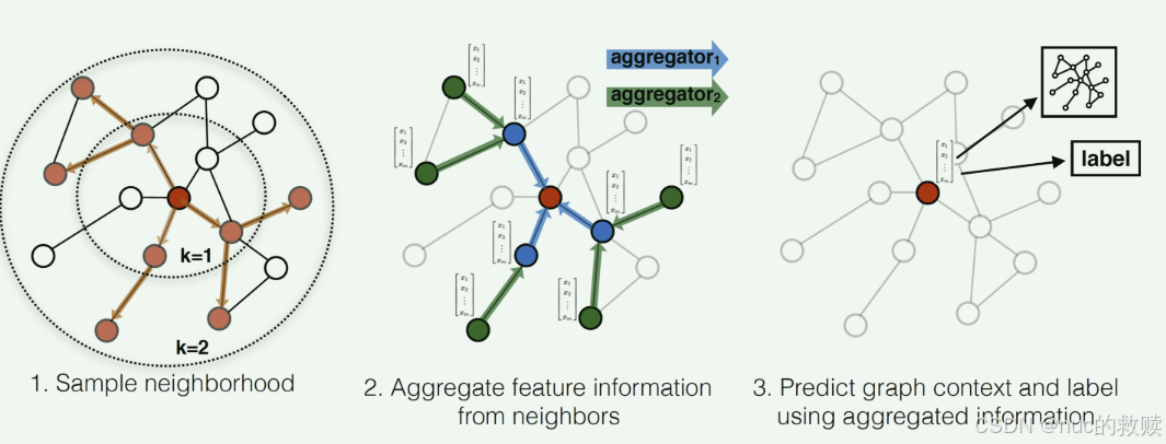
生成节点嵌入的公式:
更新过程:
(1)为了更新红色节点,首先在第一层(k=1)我们会将蓝色节点的信息聚合到红色节点上,将绿色节点的信息聚合到蓝色节点上。
所有的节点都有了新的包含邻居节点的embedding。
(2)在第二层(k=2)红色节点的embedding被再次更新,不过这次用的是更新后的蓝色节点embedding,这样就保证了红色节点更新后的embedding包括蓝色和绿色节点的信息。这样,每个节点又有了新的embedding向量,且包含更多的信息。
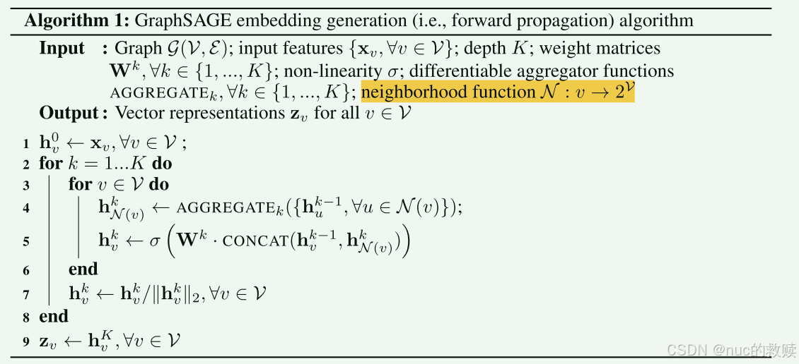
简而言之就是聚合K层采样过的邻居的特征再拼接上自己的特征,用来更新自己新的特征。
-
聚合函数:
1.mean:

2.pool:

-
小批量向前传播公式:
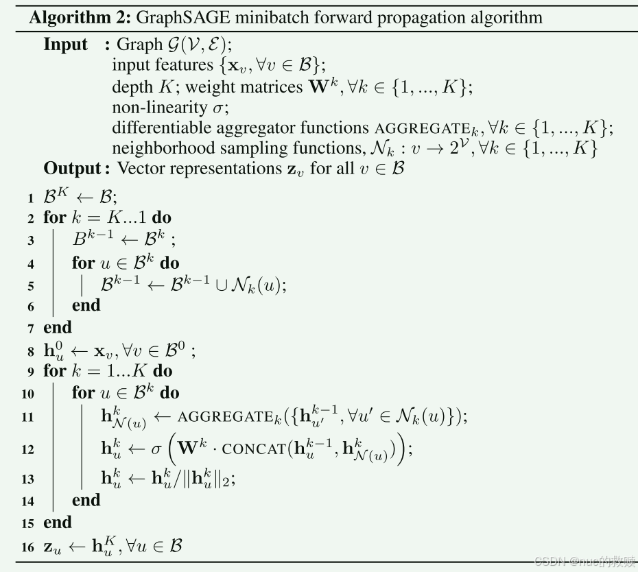
和上面的算法1一样,只不过是1-7行添加了一个采样的过程,而
不是选取所有的邻居节点了。
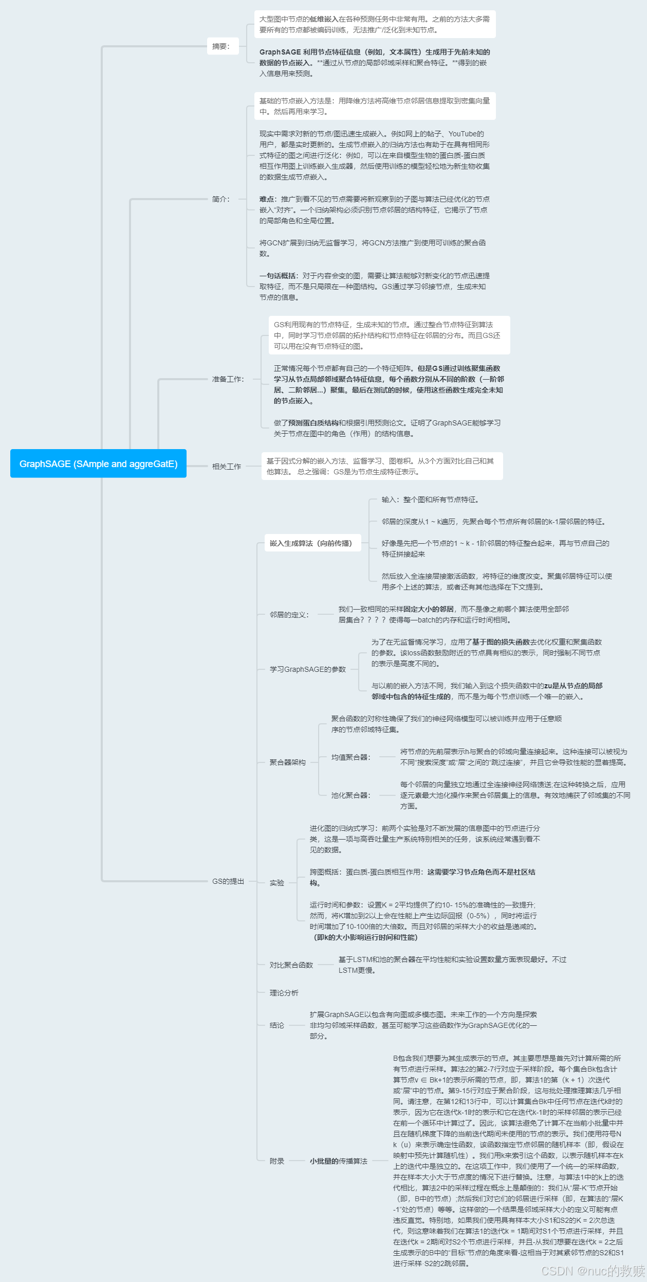
3.论文导图
4.核心代码

从中心节点开始,逐层向外寻找邻居节点然后采样,然后继续
##导入训练的batch节点
        lower_layer_nodes = list(nodes_batch)
        ##聚合节点的层
        nodes_batch_layers = [(lower_layer_nodes,)]  //存储每一层的节点

        # 每一层的graph sage
        for i in range(self.num_layers):
        ##获得邻接节点
            lower_samp_neighs, lower_layer_nodes_dict, lower_layer_nodes = self._get_unique_neighs_list(lower_layer_nodes)
        ##形成layer2(最外层节点),layer1(中间层节点),layer center(中心节点),即
            nodes_batch_layers.insert(0, (lower_layer_nodes, lower_samp_neighs, lower_layer_nodes_dict))
##获得节点的邻居
def _get_unique_neighs_list(self, nodes, num_sample=10):
_set = set
##获取每个节点的邻居节点
to_neighs = [self.adj_lists[int(node)] for node in nodes]
##进行采样
if not num_sample is None:
_sample = random.sample
##如果邻居节点个数大于等于十个,则随机取十个,如果邻居节点个数小于十个则全取
samp_neighs = [_set(_sample(to_neigh, num_sample)) if len(to_neigh) >= num_sample else to_neigh for to_neigh in to_neighs]
else:
samp_neighs = to_neighs
##将采样的邻居节点和本身的中心节点结合得到节点所属邻居的集合
samp_neighs = [samp_neigh | set([nodes[i]]) for i, samp_neigh in enumerate(samp_neighs)]
##进行去重操作
_unique_nodes_list = list(set.union(*samp_neighs))
##进行重新排列
i = list(range(len(_unique_nodes_list)))
##对字典进行重新编号
unique_nodes = dict(list(zip(_unique_nodes_list, i)))
##返回所有节点的邻居,返回所有节点的编号,返回所有节点的列表
return samp_neighs, unique_nodes, _unique_nodes_list
从次外层向里聚集
##将节点特征赋予到变量pre_hidden_embs
        pre_hidden_embs = self.raw_features
        ##nodes_batch_layers=[layer2,layer1,layer_center]
        for index in range(1, self.num_layers+1):
        ##以layer1节点作为中心节点
            nb = nodes_batch_layers[index][0]
        ##取中心节点对应的上层(layer2)的邻居节点
            pre_neighs = nodes_batch_layers[index-1]

        ##聚合函数进行聚合得到中心节点特征
            aggregate_feats = self.aggregate(nb, pre_hidden_embs, pre_neighs)
            sage_layer = getattr(self, 'sage_layer'+str(index))

        ##如果层数大于1
            if index > 1:
                nb = self._nodes_map(nb, pre_hidden_embs, pre_neighs)
        ##利用中心节点表征和聚合后的中心节点特征进行拼接然后连一个可学习的权重参数
            cur_hidden_embs = sage_layer(self_feats=pre_hidden_embs[nb],
                                        aggregate_feats=aggregate_feats)
            pre_hidden_embs = cur_hidden_embs
        return pre_hidden_embs  //graphsage层最后返回一个聚合后的节点嵌入,作为分类器的输入。
def aggregate(self, nodes, pre_hidden_embs, pre_neighs, num_sample=10):
##取出最外层邻居节点(layer2)
unique_nodes_list, samp_neighs, unique_nodes = pre_neighs
assert len(nodes) == len(samp_neighs)
##判断邻居节点是否包含了中心节点
indicator = [(nodes[i] in samp_neighs[i]) for i in range(len(samp_neighs))]
assert (False not in indicator)
##将邻居节点包含中心节点的部分去掉
if not self.gcn:
samp_neighs = [(samp_neighs[i]-set([nodes[i]])) for i in range(len(samp_neighs))
##判断如果涉及到所有中心节点,保留原先矩阵,如果不涉及所有中心,保留部分矩阵
if len(pre_hidden_embs) == len(unique_nodes):
embed_matrix = pre_hidden_embs
else:
embed_matrix = pre_hidden_embs[torch.LongTensor(unique_nodes_list)]
##以邻接节点为行,以中心节点为列构建邻接矩阵
mask = torch.zeros(len(samp_neighs), len(unique_nodes))
column_indices = [unique_nodes[n] for samp_neigh in samp_neighs for n in samp_neigh]
row_indices = [i for i in range(len(samp_neighs)) for j in range(len(samp_neighs[i]))]
##将其有链接的地方记为1
mask[row_indices, column_indices] = 1
##选择平均的方式进行聚合
if self.agg_func == 'MEAN':
##按行求和得到每个中心节点的连接的邻居节点的个数
num_neigh = mask.sum(1, keepdim=True)
##按行进行归一化操作
mask = mask.div(num_neigh).to(embed_matrix.device)
##矩阵相乘,相当于聚合周围临界信息并求和
aggregate_feats = mask.mm(embed_matrix)
elif self.agg_func == 'MAX':
# print(mask)
indexs = [x.nonzero() for x in mask==1]
aggregate_feats = []
# self.dc.logger.info('5')
for feat in [embed_matrix[x.squeeze()] for x in indexs]:
if len(feat.size()) == 1:
aggregate_feats.append(feat.view(1, -1))
else:
aggregate_feats.append(torch.max(feat,0)[0].view(1, -1))
aggregate_feats = torch.cat(aggregate_feats, 0)
# self.dc.logger.info('6')
return aggregate_feats-
分类器把 经过graphsage层采样聚集后的特征作为输入,一共有labels类,得到一个概率。然后经过有监督/无监督loss函数训练。
##定义分类器
class Classification(nn.Module):
    def __init__(self, emb_size, num_classes):
        super(Classification, self).__init__()
        #self.weight = nn.Parameter(torch.FloatTensor(emb_size, num_classes))
        self.layer = nn.Sequential(
                                nn.Linear(emb_size, num_classes)
                                #nn.ReLU())
        self.init_params()
    def init_params(self):
        for param in self.parameters():
            if len(param.size()) == 2:
                nn.init.xavier_uniform_(param)

    def forward(self, embeds):
        logists = torch.log_softmax(self.layer(embeds), 1)
        return logists
## 分类器训练
def train_classification(dataCenter, graphSage, classification, ds, device, max_vali_f1, name, epochs=800):
print('Training Classification ...')
c_optimizer = torch.optim.SGD(classification.parameters(), lr=0.5)
# train classification, detached from the current graph
#classification.init_params()
b_sz = 50
train_nodes = getattr(dataCenter, ds+'_train')
labels = getattr(dataCenter, ds+'_labels')
features = get_gnn_embeddings(graphSage, dataCenter, ds) #得到之前采样聚集后的节点特征
for epoch in range(epochs):
train_nodes = shuffle(train_nodes)
batches = math.ceil(len(train_nodes) / b_sz)
visited_nodes = set()
for index in range(batches):
nodes_batch = train_nodes[index*b_sz:(index+1)*b_sz]
visited_nodes |= set(nodes_batch)
labels_batch = labels[nodes_batch]
embs_batch = features[nodes_batch]
logists = classification(embs_batch)
loss = -torch.sum(logists[range(logists.size(0)), labels_batch], 0)
loss /= len(nodes_batch)
loss.backward()
nn.utils.clip_grad_norm_(classification.parameters(), 5)
c_optimizer.step()
c_optimizer.zero_grad()
max_vali_f1 = evaluate(dataCenter, ds, graphSage, classification, device, max_vali_f1, name, epoch) ##evaluate函数得到。。
return classification, max_vali_f1-
无监督loss
class UnsupervisedLoss(object):
    """docstring for UnsupervisedLoss"""
    def __init__(self, adj_lists, train_nodes, device):
        super(UnsupervisedLoss, self).__init__()
        self.Q = 10
        self.N_WALKS = 6
        self.WALK_LEN = 1
        self.N_WALK_LEN = 5
        self.MARGIN = 3
        self.adj_lists = adj_lists
        self.train_nodes = train_nodes
        self.device = device

        self.target_nodes = None
        self.positive_pairs = []
        self.negtive_pairs = []
        self.node_positive_pairs = {}
        self.node_negtive_pairs = {}
        self.unique_nodes_batch = []

    def get_loss_sage(self, embeddings, nodes):
    ## 确保输入的嵌入(embeddings)和唯一节点批次(unique_nodes_batch)的长度相同
        assert len(embeddings) == len(self.unique_nodes_batch)
        assert False not in [nodes[i]==self.unique_nodes_batch[i] for i in range(len(nodes))]
    ##建立节点和嵌入列表的索引的映射关系
        node2index = {n:i for i,n in enumerate(self.unique_nodes_batch)}

    ##对每个节点,计算它的正负样本对的分数
        nodes_score = []
        assert len(self.node_positive_pairs) == len(self.node_negtive_pairs)
        for node in self.node_positive_pairs:
            pps = self.node_positive_pairs[node]
            nps = self.node_negtive_pairs[node]
            if len(pps) == 0 or len(nps) == 0:
                continue
        ## 负样本对的损失,使用余弦相似度和对数sigmoid函数
            # Q * Exception(negative score)
            indexs = [list(x) for x in zip(*nps)]
            node_indexs = [node2index[x] for x in indexs[0]]
            neighb_indexs = [node2index[x] for x in indexs[1]]
            neg_score = F.cosine_similarity(embeddings[node_indexs], embeddings[neighb_indexs])
            neg_score = self.Q*torch.mean(torch.log(torch.sigmoid(-neg_score)), 0)
            #print(neg_score)

        ## 正样本对的损失,同样使用余弦相似度和对数sigmoid函数。
            # multiple positive score
            indexs = [list(x) for x in zip(*pps)]
            node_indexs = [node2index[x] for x in indexs[0]]
            neighb_indexs = [node2index[x] for x in indexs[1]]
            pos_score = F.cosine_similarity(embeddings[node_indexs], embeddings[neighb_indexs])
            pos_score = torch.log(torch.sigmoid(pos_score))
            #print(pos_score)

            nodes_score.append(torch.mean(- pos_score - neg_score).view(1,-1))

        loss = torch.mean(torch.cat(nodes_score, 0))
        return loss

##边缘损失(margin loss)
    ##这个方法与get_loss_sage类似,但在计算损失时使用了边缘损失
    def get_loss_margin(self, embeddings, nodes):
        assert len(embeddings) == len(self.unique_nodes_batch)
        assert False not in [nodes[i]==self.unique_nodes_batch[i] for i in range(len(nodes))]
        node2index = {n:i for i,n in enumerate(self.unique_nodes_batch)}

        nodes_score = []
        assert len(self.node_positive_pairs) == len(self.node_negtive_pairs)
        for node in self.node_positive_pairs:
            pps = self.node_positive_pairs[node]
            nps = self.node_negtive_pairs[node]
            if len(pps) == 0 or len(nps) == 0:
                continue
        ##正样本对的最小得分
            indexs = [list(x) for x in zip(*pps)]
            node_indexs = [node2index[x] for x in indexs[0]]
            neighb_indexs = [node2index[x] for x in indexs[1]]
            pos_score = F.cosine_similarity(embeddings[node_indexs], embeddings[neighb_indexs])
            pos_score, _ = torch.min(torch.log(torch.sigmoid(pos_score)), 0)
        ## 负样本对的最大得分
            indexs = [list(x) for x in zip(*nps)]
            node_indexs = [node2index[x] for x in indexs[0]]
            neighb_indexs = [node2index[x] for x in indexs[1]]
            neg_score = F.cosine_similarity(embeddings[node_indexs], embeddings[neighb_indexs])
            neg_score, _ = torch.max(torch.log(torch.sigmoid(neg_score)), 0)

        ##计算它们之间的差异,加上一个边缘值
            nodes_score.append(torch.max(torch.tensor(0.0).to(self.device), neg_score-pos_score+self.MARGIN).view(1,-1))
            # nodes_score.append((-pos_score - neg_score).view(1,-1))

        loss = torch.mean(torch.cat(nodes_score, 0),0)

        # loss = -torch.log(torch.sigmoid(pos_score))-4*torch.log(torch.sigmoid(-neg_score))
        return loss

    def extend_nodes(self, nodes, num_neg=6):
    ##清空当前的正负样本对和它们的映射
        self.positive_pairs = []
        self.node_positive_pairs = {}
        self.negtive_pairs = []
        self.node_negtive_pairs = {}
    ##设置目标节点为传入的节点
        self.target_nodes = nodes
    ##方法来生成正负样本对。
        self.get_positive_nodes(nodes)
        # print(self.positive_pairs)
        self.get_negtive_nodes(nodes, num_neg)
        # print(self.negtive_pairs)
    ##所有正负样本对中出现的唯一节点
        self.unique_nodes_batch = list(set([i for x in self.positive_pairs for i in x]) | set([i for x in self.negtive_pairs for i in x]))
        assert set(self.target_nodes) < set(self.unique_nodes_batch)
        return self.unique_nodes_batch
    ##正样本生成——_run_random_walks方法生成正样本对
    def get_positive_nodes(self, nodes):
        return self._run_random_walks(nodes)
    ## 每个节点生成指定数量的负样本。这些负样本是从不是节点邻居的节点中随机选取的
    def get_negtive_nodes(self, nodes, num_neg):
        for node in nodes:
            neighbors = set([node])
            frontier = set([node])
            for i in range(self.N_WALK_LEN):
                current = set()
                for outer in frontier:
                    current |= self.adj_lists[int(outer)]
                frontier = current - neighbors
                neighbors |= current
            far_nodes = set(self.train_nodes) - neighbors
            neg_samples = random.sample(far_nodes, num_neg) if num_neg < len(far_nodes) else far_nodes
            self.negtive_pairs.extend([(node, neg_node) for neg_node in neg_samples])
            self.node_negtive_pairs[node] = [(node, neg_node) for neg_node in neg_samples]
        return self.negtive_pairs
    ##随机游走函数
    def _run_random_walks(self, nodes):
        for node in nodes:
            if len(self.adj_lists[int(node)]) == 0:
                continue
            cur_pairs = []
        ##对于传入的每个节点,进行指定次数的随机游走。
            for i in range(self.N_WALKS):
                curr_node = node
                ##对于每次随机游走进行指定长度并且每次随机游走都选择邻居节点作为下一个节点
                for j in range(self.WALK_LEN):
                    neighs = self.adj_lists[int(curr_node)]
                    next_node = random.choice(list(neighs))
                    # self co-occurrences are useless
                    ##如果选中的邻居节点不是原始节点且在训练节点集中,将其作为正样本对添加到列表中
                    if next_node != node and next_node in self.train_nodes:
                        self.positive_pairs.append((node,next_node))
                        cur_pairs.append((node,next_node))
                    curr_node = next_node

            self.node_positive_pairs[node] = cur_pairs
        return self.positive_pairs
正负样本定义
什么是正负样本?事实上,在目标检测领域正负样本的定义策略是不断变化的。正负样本是在训练过程中计算损失用的,而在预测过程和验证过程是没有这个概念的。许多人在看相关目标检测的论文时,常常误以为正样本就是我们手动标注的GT,其实不然。
首先,
正样本是待检测的目标,比如检测人脸时,人脸是正样本,非人脸则是负样本,比如旁边的树呀花呀之类的其他东西;其次,正负样本都是针对于算法经过处理生成的框(如:计算宽高比、交并比、样本扩充等)而言,而非原始的GT数据。
随机游走算法的基本思想是:
从一个或一系列顶点开始遍历一张图。在任意一个顶点,遍历者将以概率1-a游走到这个顶点的邻居顶点,以概率a随机跳跃到图中的任何一个顶点,称a为跳转发生概率,每次游走后得出一个概率分布,该概率分布刻画了图中每一个顶点被访问到的概率。用这个概率分布作为下一次游走的输入并反复迭代这一过程。当满足一定前提条件时,这个概率分布会趋于收敛。收敛后,即可以得到一个平稳的概率分布。
5.整体总结一下
GraphSAGE是一种能利用顶点的属性信息高效
产生未知顶点embedding的一种归纳式(inductive)学习的框架。
主要步骤:
(1)对邻居随机采样
(2)使用聚合函数将采样的邻居节点的Embedding进行聚合,用于更新节点的embedding。
(3)根据更新后的embedding预测节点的标签。
6.核心思想 / 贡献
只要有边就能聚合信息,改进gcn,不再需要邻接矩阵
与gcn不同的消息传递方法,不依赖邻接矩阵,而是
边索引
mini batch的使用,改进gcn的全图训练。
7.问:如何生成未知节点(测试集)embedding的?
答:假如在这个图里面,存在新生成的节点,例如社交网络或者蛋白质结构rna结构之类的情况。用之前的图训练好的模型,
根据之前训练好的参数和新节点的特征,再用上面的流程,生成新节点的embedding。


 7935
7935

 被折叠的 条评论
为什么被折叠?
被折叠的 条评论
为什么被折叠?
 到【灌水乐园】发言


