PyTorch|简单实现线性回归模型

01 | 什么是线性回归？

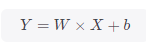
线性回归是分析一个变量与另外一个（或多个）变量之间关系的一种方法，该方法需要从实际数据中抽象出因变量Y、自变量X，且假定Y相对于X按照近似线性的方式变化，即函数图像上近似呈现一条直线。通常可以用下述公式表示，而模型求解目标为确定其中的斜率W与偏置b。

线性回归的求解过程一般分为三步：

1. 确定模型，对于我们而言即确定模型求解目标是确定W与b

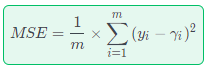
2. 选择损失函数作为优化迭代目标，本例中选用常用的均方误差指标（MSE），即模型预测值与真实值差的平方和均值，用公式表示即:
   

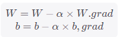
3. 最后就是求解MSE中相对于W与b的梯度并更新W与b，以获得较小MSE时的最优参数数值。
   

02 | PyCharm下的PyTorch代码

# 借助PyTorch实现一个简单的线性回归模型 
import matplotlib.pyplot as plt 
import torch 

torch.manual_seed(10) #设定随机数种子 
lr = 0.1 # 学习率 

# 创建训练集 
x = torch.rand(20, 1) * 10 # 创建一个（20,1）的Tensor，每个数值扩大10倍（默认小于1） 
y = 2*x + (6 + torch.randn(20, 1)) # 近似线性公式，模拟随机噪声 

# 构建线性回归参数张量
w = torch.randn((1), requires_grad=True) 
b = torch.zeros((1), requires_grad=True) 

for iteration in range(10000):    
		# 前向传播        
		wx = torch.mul(w, x)        
		y_pred = torch.add(wx, b)            

		# 计算MSE Loss        
		loss = (0.5 * (y - y_pred) ** 2).mean()            

		# 反向传播        
		loss.backward()            

		# 更新参数        
		b.data.sub_(lr * b.grad)        
		w.data.sub_(lr * w.grad)            

		# 绘图        
		if iteration % 20 == 0:            
		plt.scatter(x.data.numpy(), y.data.numpy())                
		plt.plot(x.data.numpy(), y_pred.data.numpy(), 'r-', lw=5)                
		plt.text(2, 20, 'Loss-%.4f' % loss.data.numpy(), fontdict={'size': 20, 'color': 'red'})                
		plt.xlim(1.5, 10)                
		plt.ylim(8, 28)                
		plt.title("Iteration: {}\nw:{} b:{}".format(iteration, w.data.numpy(), b.data.numpy()))                
		plt.pause(0.5)                        

		if loss.data.numpy() < 1:                    
				break

这里将目标参数看作是1维张量，从而具有了求解梯度相关的属性值，如果依次打印出迭代更新后的W与b，可以发现其逐步迭代变化：

0 : w: tensor([4.7343], requires_grad=True) b: tensor([0.4637], requires_grad=True)1 : w: tensor([1.1161], requires_grad=True) b: tensor([0.0062], requires_grad=True)
2 : w: tensor([3.8857], requires_grad=True) b: tensor([0.6501], requires_grad=True)
3 : w: tensor([3.3481], requires_grad=True) b: tensor([0.8179], requires_grad=True)
4 : w: tensor([1.2252], requires_grad=True) b: tensor([0.7864], requires_grad=True)
5 : w: tensor([4.6958], requires_grad=True) b: tensor([1.7186], requires_grad=True)
6 : w: tensor([1.5425], requires_grad=True) b: tensor([1.6252], requires_grad=True)
7 : w: tensor([2.4540], requires_grad=True) b: tensor([2.2383], requires_grad=True)
8 : w: tensor([4.0204], requires_grad=True) b: tensor([2.9985], requires_grad=True)
9 : w: tensor([0.5421], requires_grad=True) b: tensor([2.9742], requires_grad=True)
10 : w: tensor([3.7664], requires_grad=True) b: tensor([4.0679], requires_grad=True)
。。。 。。。
98 : w: tensor([0.4375], requires_grad=True) b: tensor([8.0425], requires_grad=True)
99 : w: tensor([1.6515], requires_grad=True) b: tensor([7.6664], requires_grad=True)
100 : w: tensor([3.2623], requires_grad=True) b: tensor([7.3332], requires_grad=True)

03 | 绘图展示

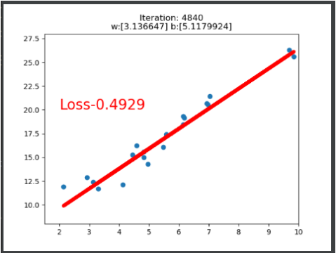
通过运行上述代码，可以实时每20次查看一次迭代情况，分别展示如下：可以看到经过100次迭代后，当MSE=0.897时，符合小于1条件，迭代终止，此时所得的直线已经近似于我们给定的线性模型。

经过调整阈值为0.5，迭代1000次后可以得到更好的结果：

4840 : w: tensor([3.1366], requires_grad=True) b: tensor([5.1180], requires_grad=True)