


python手写模拟梯度下降
以2元线性回归为例实现分类器:
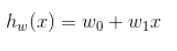
线性回归函数:
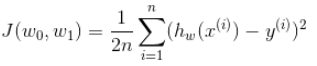
误差函数(损失函数):
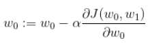
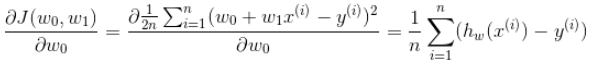
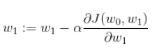
每次梯度下降参数的变化:

使用TensorFlow框架
import tensorflow as tf
import numpy as np
import matplotlib.pyplot as plt


def add_layer(input, in_size, out_size, activation_function=None):
    Weight = tf.Variable(tf.random_normal([in_size, out_size]))
    biases = tf.Variable(tf.zeros([1, out_size]))
    y = tf.matmul(input, Weight) + biases
    if activation_function is None:
        return y
    else:
        return activation_function(y)


X_data = np.linspace(-1, 1, 100, dtype=np.float32)[:, np.newaxis]
noise = np.random.normal(0, 0.05, (X_data.shape[0], 1))
# 使得产生的数据在x^2+0.5曲线上下
y_data = np.square(X_data) + 0.5 + noise

X = tf.placeholder(tf.float32, [None, 1])
y = tf.placeholder(tf.float32, [None, 1])

# 通过add_layer指定了该层框架,之后在迭代过程中不再调用函数
# 输入层为1个神经元,隐藏层为10个神经元,输出层为1个神经元
hidden_layer = add_layer(X, 1, 10, activation_function=tf.nn.relu)
output_layer = add_layer(hidden_layer, 10, 1, activation_function=None)

loss = tf.reduce_mean(tf.square(y - output_layer))
trainer = tf.train.GradientDescentOptimizer(0.1).minimize(loss)

fig, ax = plt.subplots(1, 1)
ax.scatter(X_data, y_data)
with tf.Session() as sess:
    sess.run(tf.global_variables_initializer())
    for _ in range(301):
        sess.run(trainer, feed_dict={X: X_data, y: y_data})
        if _ % 50 == 0:
            print(sess.run(loss, feed_dict={X: X_data, y: y_data}))
            curve = ax.plot(X_data, sess.run(output_layer, feed_dict={X: X_data, y: y_data}))
            plt.pause(0.5)  # 停留0.5s
            if _ != 300:
                ax.lines.remove(curve[0])  # 抹除ax上的线,必须以列表下标的形式


plt.show()
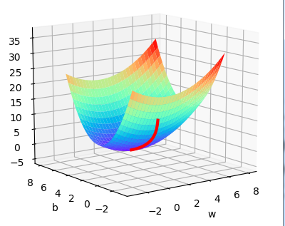
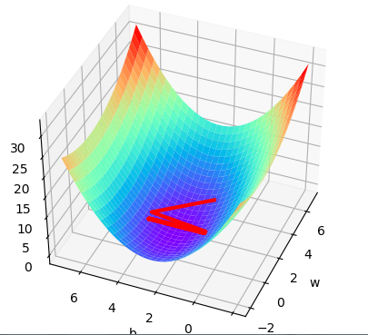
线性回归,梯度下降算法可视化:
import tensorflow as tf
import numpy as np
import matplotlib.pyplot as plt
from mpl_toolkits.mplot3d import Axes3D

lr = 0.1
real_params = [1.2, 2.5]   # 真正的参数


tf_X = tf.placeholder(tf.float32, [None, 1])
tf_y = tf.placeholder(tf.float32, [None, 1])
weight = tf.Variable(initial_value=[[5]], dtype=tf.float32)
bia = tf.Variable(initial_value=[[4]], dtype=tf.float32)
y = tf.matmul(tf_X, weight) + bia

loss = tf.losses.mean_squared_error(tf_y, y)
train_op = tf.train.GradientDescentOptimizer(lr).minimize(loss)

X_data = np.linspace(-1, 1, 200)[:, np.newaxis]
noise = np.random.normal(0, 0.1, X_data.shape)
y_data = X_data * real_params[0] + real_params[1] + noise

sess = tf.Session()
sess.run(tf.global_variables_initializer())

weights = []
biases = []
losses = []
for step in range(400):
    w, b, cost, _ = sess.run([weight, bia, loss, train_op],
                             feed_dict={tf_X: X_data, tf_y: y_data})
    weights.append(w)
    biases.append(b)
    losses.append(cost)
result = sess.run(y, feed_dict={tf_X: X_data, tf_y: y_data})

plt.figure(1)
plt.scatter(X_data, y_data, color='r', alpha=0.5)
plt.plot(X_data, result, lw=3)

fig = plt.figure(2)
ax_3d = Axes3D(fig)
w_3d, b_3d = np.meshgrid(np.linspace(-2, 7, 30), np.linspace(-2, 7, 30))
loss_3d = np.array(
    [np.mean(np.square((X_data * w_ + b_) - y_data))
     for w_, b_ in zip(w_3d.ravel(), b_3d.ravel())]).reshape(w_3d.shape)
ax_3d.plot_surface(w_3d, b_3d, loss_3d, cmap=plt.get_cmap('rainbow'))
weights = np.array(weights).ravel()
biases = np.array(biases).ravel()

# 描绘初始点
ax_3d.scatter(weights[0], biases[0], losses[0], s=30, color='r')
ax_3d.set_xlabel('w')
ax_3d.set_ylabel('b')
ax_3d.plot(weights, biases, losses, lw=3, c='r')
plt.show()
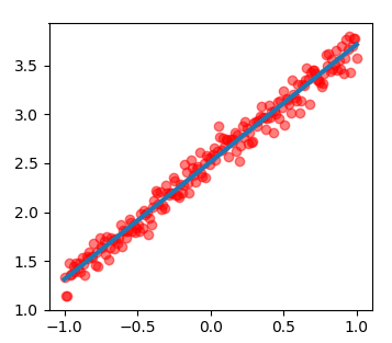
拟合线性函数:y=1.2 x + 2.5
设初始的参数w=5,b=4,lr=0.1的拟合图像和梯度下降图像:
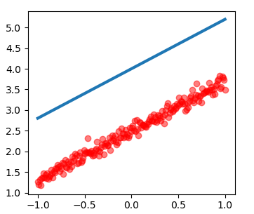
更改学习速率lr=1.0的图像:


 6796
6796


 被折叠的 条评论
为什么被折叠?
被折叠的 条评论
为什么被折叠?
 到【灌水乐园】发言


