Radial basis function(径向基函数->(高斯核函数))

最新推荐文章于 2024-03-17 22:57:36 发布

witnessai1

最新推荐文章于 2024-03-17 22:57:36 发布

阅读量1.9w

点赞数 6

分类专栏： ——机器学习—— 文章标签：机器学习高斯核函数径向基函数支持向量机算法

本文链接：https://blog.csdn.net/witnessai1/article/details/49864735

版权

——机器学习—— 专栏收录该内容

37 篇文章 0 订阅

订阅专栏

中文简单介绍:

在机器学习中，（高斯）径向基函数核（英语：Radial basis function kernel），或称为RBF核，是一种常用的核函数。它是支持向量机分类中最为常用的核函数。^[1]

关于两个样本x和x'的RBF核可表示为某个“输入空间”（input space）的特征向量，它的定义如下所示：^[2]

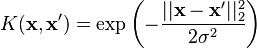
K(\mathbf{x}, \mathbf{x'}) = \exp\left(-\frac{||\mathbf{x} - \mathbf{x'}||_2^2}{2\sigma^2}\right)

$\textstyle||\mathbf{x} - \mathbf{x'}||_2^2$ 可以看做两个特征向量之间的平方欧几里得距离。 $\sigma$ 是一个自由参数。一种等价但更为简单的定义是设一个新的参数 $\gamma$ ，其表达式为 $\textstyle\gamma = -\tfrac{1}{2\sigma^2}$ ：

K(\mathbf{x}, \mathbf{x'}) = \exp(\gamma||\mathbf{x} - \mathbf{x'}||_2^2)

因为RBF核函数的值随距离减小，并介于0（极限）和1（当x = x'的时候）之间，所以它是一种现成的相似性度量表示法。^[2]核的特征空间有无穷多的维数；对于 $\sigma = 1$ ，它的展开式为：^[3]

\exp\left(-\frac{1}{2}||\mathbf{x} - \mathbf{x'}||_2^2\right) = \sum_{j=0}^\infty \frac{(\mathbf{x}^\top \mathbf{x'})^j}{j!} \exp\left(-\frac{1}{2}||\mathbf{x}||_2^2\right) \exp\left(-\frac{1}{2}||\mathbf{x'}||_2^2\right)

近似[编辑]

因为支持向量机和其他模型使用了核技巧，它在处理输入空间中大量的训练样本或含有大量特征的样本的时表现不是很好。所以，目前已经设计出了多种RBF核（或相似的其他核）的近似方法。^[4] 典型的情况下，这些方法使用z(x)的形式，也就是用一个函数对一个与其他向量（例如支持向量机中的支持向量）无关的单向量进行变换，例如：

z(\mathbf{x})z(\mathbf{x'}) \approx \varphi(\mathbf{x})\varphi(\mathbf{x'}) = K(\mathbf{x}, \mathbf{x'})

其中 $\textstyle\varphi$ 是RBF核中植入的隐式映射。

一种构造这样的z函数的方法是对核函数作傅里叶变换，然后从中随机抽出所需函数。^[5]

wiki详解：

A radial basis function (RBF) is a real-valued function whose value depends only on the distance from the origin, so that

\phi(\mathbf{x}) = \phi(\|\mathbf{x}\|)

; or alternatively on the distance from some other point c, called a center, so that

\phi(\mathbf{x}, \mathbf{c}) = \phi(\|\mathbf{x}-\mathbf{c}\|)

. Any function

\phi

that satisfies the property

\phi(\mathbf{x}) = \phi(\|\mathbf{x}\|)

is a radial function. The norm is usually Euclidean distance, although other distance functions are also possible. For example, using Łukaszyk–Karmowski metric, it is possible for some radial functions to avoid problems with ill conditioning of the matrix solved to determine coefficients w _i (see below), since the

\|\mathbf{x}\|

is always greater than zero. ^[1]

Sums of radial basis functions are typically used to approximate given functions. This approximation process can also be interpreted as a simple kind of neural network; this was the context in which they originally surfaced, in work by David Broomhead and David Lowe in 1988,^[2]^[3] which stemmed from Michael J. D. Powell's seminal research from 1977.^[4]^[5]^[6] RBFs are also used as a kernel in support vector classification.^[7]

[hide]

Types[edit]

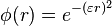
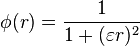
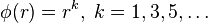
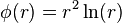
Commonly used types of radial basis functions include (writing 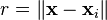$r = \|\mathbf{x} - \mathbf{x}_i\|\;$ ):

Gaussian:

The first term, that is used for normalisation of the Gaussian, is missing, because in our sum every Gaussian has a weight, so the normalisation is not necessary.

\phi(r) = e^{-(\varepsilon r)^2}\,

Multiquadric:

\phi(r) = \sqrt{1 + (\varepsilon r)^2}

Inverse quadratic:

\phi(r) = \frac{1}{1+(\varepsilon r)^2}

Inverse multiquadric:

\phi(r) = \frac{1}{\sqrt{1 + (\varepsilon r)^2}}

Polyharmonic spline:

\phi(r) = r^k,\; k=1,3,5,\dots

\phi(r) = r^k \ln(r),\; k=2,4,6,\dots

Thin plate spline (a special polyharmonic spline):

\phi(r) = r^2 \ln(r)\;

Approximation[edit]

Main article: Kernel smoothing

Radial basis functions are typically used to build up function approximations of the form

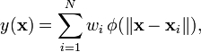
y(\mathbf{x}) = \sum_{i=1}^N w_i \, \phi(\|\mathbf{x} - \mathbf{x}_i\|),

where the approximating function y(x) is represented as a sum of N radial basis functions, each associated with a different center x_i, and weighted by an appropriate coefficient w_i. The weights w_i can be estimated using the matrix methods of linear least squares, because the approximating function is linear in the weights.

Approximation schemes of this kind have been particularly used^{[citation needed]} in time series prediction and control of nonlinear systems exhibiting sufficiently simple chaotic behaviour, 3D reconstruction in computer graphics (for example, hierarchical RBF and Pose Space Deformation).

RBF Network[edit]

Main article: radial basis function network

Two unnormalized Gaussian radial basis functions in one input dimension. The basis function centers are located at x ₁=0.75 and x ₂=3.25.

The sum

y(\mathbf{x}) = \sum_{i=1}^N w_i \, \phi(\|\mathbf{x} - \mathbf{x}_i\|),

can also be interpreted as a rather simple single-layer type of artificial neural network called a radial basis function network, with the radial basis functions taking on the role of the activation functions of the network. It can be shown that any continuous function on a compact interval can in principle be interpolated with arbitrary accuracy by a sum of this form, if a sufficiently large number N of radial basis functions is used.

The approximant y(x) is differentiable with respect to the weights w_i. The weights could thus be learned using any of the standard iterative methods for neural networks.

Using radial basis functions in this manner yields a reasonable interpolation approach provided that the fitting set has been chosen such that it covers the entire range systematically (equidistant data points are ideal). However, without a polynomial term that is orthogonal to the radial basis functions, estimates outside the fitting set tend to perform poorly.

References[edit]

Jump up^ Łukaszyk, S. (2004) A new concept of probability metric and its applications in approximation of scattered data sets. Computational Mechanics, 33, 299-3004. limited access
Jump up^Radial Basis Function networks
Jump up^ Broomhead, David H.; Lowe, David (1988). "Multivariable Functional Interpolation and Adaptive Networks" (PDF). Complex Systems 2: 321––355. Archived from the original (PDF) on 2014-07-14.
Jump up^ Michael J. D. Powell (1977). "Restart procedures for the conjugate gradient method" (PDF). Mathematical Programming (Springer) 12 (1): 241––254.
Jump up^ Sahin, Ferat (1997). A Radial Basis Function Approach to a Color Image Classification Problem in a Real Time Industrial Application (PDF) (M.Sc.). Virginia Tech. p. 26. Radial basis functions were first introduced by Powell to solve the real multivariate interpolation problem.
Jump up^ Broomhead & Lowe 1988, p. 347: "We would like to thank Professor M.J.D. Powell at the Department of Applied Mathematics and Theoretical Physics at Cambridge University for providing the initial stimulus for this work."
Jump up^ VanderPlas, Jake (6 May 2015). "Introduction to Support Vector Machines" [O'Reilly]. Retrieved 14 May 2015.