Machine Learning week 5 programming exercise Neural Network Learning

Neural Networks Learning

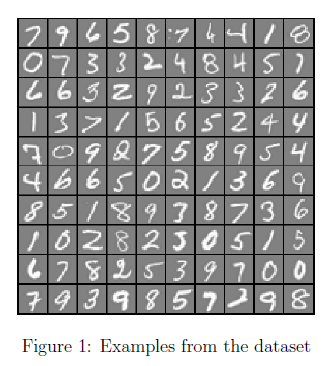
Visualizing the data

这次试用的数据和上次是一样的数据。5000个training example，每一个代表一个数字的图像，图像是20x20的灰度图，400个像素的每个位置的灰度值组成了一个training example。

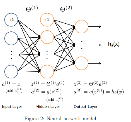
Model representation

这里我们使用如下的模型，共3层，其中第一层input有400个feature，另外还有bias unit。

这个练习中实现训练了一些theta，通过如下的代码把theta1和theta2读取出来

[cpp]  view plain  copy

1. % Load saved matrices from file  
2. load('ex4weights.mat');  
3. % The matrices Theta1 and Theta2 will now be in your workspace  
4. % Theta1 has size 25 x 401  
5. % Theta2 has size 10 x 26  

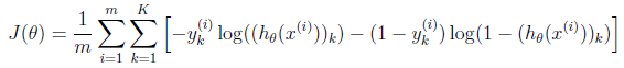
Feedforward and cost function

现在我们需要计算cost function和gradient

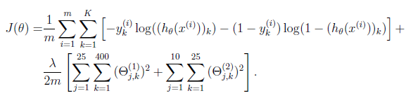
这里是没有regularization的情况下的cost function公式，m表示m个training example，k表示k个output，这里我们有10个output，分别代表1-10

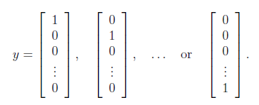
y的值需要从数字形式转化为向量形式，如下，下面的例子中第一列表示1，第二列表示2

Regularized cost function

下面是regularized cost function，其实就是在普通的cost function后面加上每个theta的平方，当然不要忘了系数。不过这里并不是所有的theta，所有跟bias unit相关的theta都要排除。

我们现在这里写的程序，指针对3层网络，但是对于由于每层unit数量不一样出现的不同的网络，我们这里也要兼容

[cpp]  view plain  copy

1. function [J grad] = nnCostFunction(nn_params, ...  
2.                                    input_layer_size, ...  
3.                                    hidden_layer_size, ...  
4.                                    num_labels, ...  
5.                                    X, y, lambda)  
6. %NNCOSTFUNCTION Implements the neural network cost function for a two layer  
7. %neural network which performs classification  
8. %   [J grad] = NNCOSTFUNCTON(nn_params, hidden_layer_size, num_labels, ...  
9. %   X, y, lambda) computes the cost and gradient of the neural network. The  
10. %   parameters for the neural network are "unrolled" into the vector  
11. %   nn_params and need to be converted back into the weight matrices.   
12. %   
13. %   The returned parameter grad should be a "unrolled" vector of the  
14. %   partial derivatives of the neural network.  
15. %  
16.   
17. % Reshape nn_params back into the parameters Theta1 and Theta2, the weight matrices  
18. % for our 2 layer neural network  
19. Theta1 = reshape(nn_params(1:hidden_layer_size * (input_layer_size + 1)), ...  
20.                  hidden_layer_size, (input_layer_size + 1));  
21.   
22. Theta2 = reshape(nn_params((1 + (hidden_layer_size * (input_layer_size + 1))):end), ...  
23.                  num_labels, (hidden_layer_size + 1));  
24.   
25. % Setup some useful variables  
26. m = size(X, 1);  
27.            
28. % You need to return the following variables correctly   
29. J = 0;  
30. Theta1_grad = zeros(size(Theta1));  
31. Theta2_grad = zeros(size(Theta2));  
32.   
33. % ====================== YOUR CODE HERE ======================  
34. % Instructions: You should complete the code by working through the  
35. %               following parts.  
36. %  
37. % Part 1: Feedforward the neural network and return the cost in the  
38. %         variable J. After implementing Part 1, you can verify that your  
39. %         cost function computation is correct by verifying the cost  
40. %         computed in ex4.m  
41. %  
42. % Part 2: Implement the backpropagation algorithm to compute the gradients  
43. %         Theta1_grad and Theta2_grad. You should return the partial derivatives of  
44. %         the cost function with respect to Theta1 and Theta2 in Theta1_grad and  
45. %         Theta2_grad, respectively. After implementing Part 2, you can check  
46. %         that your implementation is correct by running checkNNGradients  
47. %  
48. %         Note: The vector y passed into the function is a vector of labels  
49. %               containing values from 1..K. You need to map this vector into a   
50. %               binary vector of 1's and 0's to be used with the neural network  
51. %               cost function.  
52. %  
53. %         Hint: We recommend implementing backpropagation using a for-loop  
54. %               over the training examples if you are implementing it for the   
55. %               first time.  
56. %  
57. % Part 3: Implement regularization with the cost function and gradients.  
58. %  
59. %         Hint: You can implement this around the code for  
60. %               backpropagation. That is, you can compute the gradients for  
61. %               the regularization separately and then add them to Theta1_grad  
62. %               and Theta2_grad from Part 2.  
63. %  
64. #计算每层的结果，记得要把bias unit加上，第一次写把a1 写成了 [ones(m,1); X];  
65. a1 = [ones(m,1) X];  
66. z2 = Theta1 * a1';  
67. a2 = sigmoid(z2);  
68. a2 = [ones(1,m); a2]; #这里 a2 和 a1 的格式已经不一样了，a1是行排列，a2是列排列  
69. z3 = Theta2 * a2;  
70. a3 = sigmoid(z3);  
71.   
72. # 首先把原先label表示的y变成向量模式的output，下面用了循环  
73. y_vect = zeros(num_labels, m);  
74. for i = 1:m,  
75.     y_vect(y(i),i) = 1;  
76. end;  
77.   
78. #每一training example的cost function是使用的向量计算，然后for loop累加所有m个training example  
79. #的cost function  
80. for i=1:m,  
81.     J += sum(-1*y_vect(:,i).*log(a3(:,i))-(1-y_vect(:,i)).*log(1-a3(:,i)));  
82. end;  
83. J = J/m;  
84.   
85. #增加regularization，一开始只写了一个sum，但其实theta1 2 分别都是矩阵，一个sum只能按列累加，bias unit的theta不参与regularization  
86. J = J + lambda*(sum(sum(Theta1(:,2:end).^2))+sum(sum(Theta2(:,2:end).^2)))/2/m;  
87.   
88. #backward propagation  
89. #Δ的元素个数应该和对应的theta中的元素的个数相同  
90. Delta1 = zeros(size(Theta1));  
91. Delta2 = zeros(size(Theta2));  
92. for i=1:m,  
93.     delta3 = a3(:,i) - y_vect(:,i);  
94.       
95.     #注意这里的δ是不包含bias unit的delta的，毕竟bias unit永远是1，  
96.     #不需要计算delta, 下面的2:end,: 过滤掉了bias unit相关值  
97.     delta2 = (Theta2'*delta3)(2:end,:).*sigmoidGradient(z2(:,i));  
98.     #移除bias unit上的delta2，但是由于上面sigmoidGradient式子中  
99.     #的z，本身不包含bias unit，所以下面的过滤不必要，注释掉。  
100.     #delta2 = delta2(2:end);  
101.     Delta2 += delta3 * a2(:,i)';  
102.       
103.     #第一层的input是一行一行的，和后面的结构不一样，后面是一列作为一个example  
104.     Delta1 += delta2 * a1(i,:);  
105. end;  
106.   
107. #总结一下，δ不包含bias unit的偏差值，Δ对跟θ对应的，用来计算每个θ  
108. #后面的偏导数的，所以Δ包含bias unit的θ  
109. Theta2_grad = Delta2/m;  
110. Theta1_grad = Delta1/m;  
111.   
112. #regularization gradient  
113.   
114. Theta2_grad(:,2:end) = Theta2_grad(:,2:end) .+ lambda * Theta2(:,2:end) / m;  
115. Theta1_grad(:,2:end) = Theta1_grad(:,2:end) .+ lambda * Theta1(:,2:end) / m;  
116.   
117.   
118.   
119.   
120.   
121.   
122. % -------------------------------------------------------------  
123.   
124. % =========================================================================  
125.   
126. % Unroll gradients  
127. grad = [Theta1_grad(:) ; Theta2_grad(:)];  
128.   
129.   
130. end  

Backpropagation

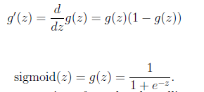
Sigmoid gradient

sigmoid gradient反向传播计算gradient的公式的一部分

[cpp]  view plain  copy

1. function g = sigmoidGradient(z)  
2. %SIGMOIDGRADIENT returns the gradient of the sigmoid function  
3. %evaluated at z  
4. %   g = SIGMOIDGRADIENT(z) computes the gradient of the sigmoid function  
5. %   evaluated at z. This should work regardless if z is a matrix or a  
6. %   vector. In particular, if z is a vector or matrix, you should return  
7. %   the gradient for each element.  
8.   
9. g = zeros(size(z));  
10.   
11. % ====================== YOUR CODE HERE ======================  
12. % Instructions: Compute the gradient of the sigmoid function evaluated at  
13. %               each value of z (z can be a matrix, vector or scalar).  
14.   
15. g = sigmoid(z).*(1-sigmoid(z));  
16.   
17. % =============================================================  
18. end  

Random initialization

为了打破symmetry breaking，我们要在选取初始theta的时候，每次选择某一层的theta，然后让每个这一层的theta都随机选取，范围 [-ξ，ξ]

有如下经验公式可用来选择合适的theta范围

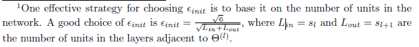
确定了范围之后，下面是随机选择的过程

[cpp]  view plain  copy

1. % Randomly initialize the weights to small values  
2. epsilon init = 0.12;  
3. W = rand(L out, 1 + L in) * 2 * epsilon init − epsilon init;  

Backpropagation

在反向传播过程中，我们要计算除了input layer之外的每层的小 delta，也就是δ。参考下图，

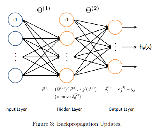
计算过程分为下面5步，每个training example都循环进行1-4：

1 forward propagation计算每一层的函数z，和每一层的activation，不要忘记途中增加bias unit

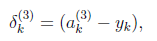
2 计算第三层的δ，

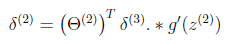
3 计算第二层的δ，

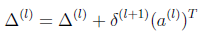
4计算每一层的Δ，这里要搞清楚，δ代表当前层的所有unit个数，如果是hidden layer的话，还包括了bias unit。Δ的最终结果是当前层的theta的偏导数，和当前层的theta维数一致，通过δ计算Δ的时候，由于后层的δ中的bias unit并不是有当前层的theta计算到的，反向计算theta的偏导数，Δ的时候则要把其中的bias unit去掉

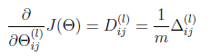
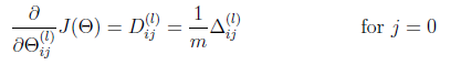
5 上面m个training example都循环计算完成之后，计算最后的偏导数

实际上这里的第一步，可以一次性使用矩阵操作计算完成所有m个训练数据的结果，但是后面的几步，还是要循环计算每个训练数据的结果

Gradient checking

这里主要是对我们上面编写的计算偏导数的函数进行验证的一个方法，通过比较上面计算结果和这里计算的估计结果的关系来判断，我们的code是否正确。

这里我们选择ε= 10^−4, 最终我们会看到我们计算的偏导数和估计的偏导数差值应该是 1e-9的数量级。

当然这里计算的时候可以使用比较少的unit的网络，因为这里估计值的计算计算量很大。

[cpp]  view plain  copy

1. function numgrad = computeNumericalGradient(J, theta)  
2. %COMPUTENUMERICALGRADIENT Computes the gradient using "finite differences"  
3. %and gives us a numerical estimate of the gradient.  
4. %   numgrad = COMPUTENUMERICALGRADIENT(J, theta) computes the numerical  
5. %   gradient of the function J around theta. Calling y = J(theta) should  
6. %   return the function value at theta.  
7.   
8. % Notes: The following code implements numerical gradient checking, and   
9. %        returns the numerical gradient.It sets numgrad(i) to (a numerical   
10. %        approximation of) the partial derivative of J with respect to the   
11. %        i-th input argument, evaluated at theta. (i.e., numgrad(i) should   
12. %        be the (approximately) the partial derivative of J with respect   
13. %        to theta(i).)  
14. %                  
15.   
16. numgrad = zeros(size(theta));  
17. perturb = zeros(size(theta));  
18. e = 1e-4;  
19. for p = 1:numel(theta)  
20.     % Set perturbation vector  
21.     perturb(p) = e;  
22.     loss1 = J(theta - perturb);  
23.     loss2 = J(theta + perturb);  
24.     % Compute Numerical Gradient  
25.     numgrad(p) = (loss2 - loss1) / (2*e);  
26.     perturb(p) = 0;  
27. end  
28.   
29. end  

Regularized Neural Networks

计算的时候，所有和bias项对应的theta都不需要做regularization

Learning parameters using fmincg

略

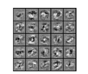
Visualizing the hidden layer

这里很有意思，我们的input是400个像素点的灰度值，而theta1的每一行都是一个401的vector，去掉第一个，同样得到一个400的vector，然后我们把它可视化出来，可以大概看到我们做了什么

change lambda

不同的λ，会得到不同的结果，怎么选取lambda呢？

[cpp]  view plain  copy

1. %% Machine Learning Online Class - Exercise 4 Neural Network Learning  
2.   
3. %  Instructions  
4. %  ------------  
5. %   
6. %  This file contains code that helps you get started on the  
7. %  linear exercise. You will need to complete the following functions   
8. %  in this exericse:  
9. %  
10. %     sigmoidGradient.m  
11. %     randInitializeWeights.m  
12. %     nnCostFunction.m  
13. %  
14. %  For this exercise, you will not need to change any code in this file,  
15. %  or any other files other than those mentioned above.  
16. %  
17.   
18. %% Initialization  
19. clear ; close all; clc  
20.   
21. %% Setup the parameters you will use for this exercise  
22. input_layer_size  = 400;  % 20x20 Input Images of Digits  
23. hidden_layer_size = 25;   % 25 hidden units  
24. num_labels = 10;          % 10 labels, from 1 to 10     
25.                           % (note that we have mapped "0" to label 10)  
26.   
27. %% =========== Part 1: Loading and Visualizing Data =============  
28. %  We start the exercise by first loading and visualizing the dataset.   
29. %  You will be working with a dataset that contains handwritten digits.  
30. %  
31.   
32. % Load Training Data  
33. fprintf('Loading and Visualizing Data ...\n')  
34.   
35. load('ex4data1.mat');  
36. m = size(X, 1);  
37.   
38. % Randomly select 100 data points to display  
39. sel = randperm(size(X, 1));  
40. sel = sel(1:100);  
41.   
42. displayData(X(sel, :));  
43.   
44. fprintf('Program paused. Press enter to continue.\n');  
45. pause;  
46.   
47.   
48. %% ================ Part 2: Loading Parameters ================  
49. % In this part of the exercise, we load some pre-initialized   
50. % neural network parameters.  
51.   
52. fprintf('\nLoading Saved Neural Network Parameters ...\n')  
53.   
54. % Load the weights into variables Theta1 and Theta2  
55. load('ex4weights.mat');  
56.   
57. % Unroll parameters   
58. nn_params = [Theta1(:) ; Theta2(:)];  
59.   
60. %% ================ Part 3: Compute Cost (Feedforward) ================  
61. %  To the neural network, you should first start by implementing the  
62. %  feedforward part of the neural network that returns the cost only. You  
63. %  should complete the code in nnCostFunction.m to return cost. After  
64. %  implementing the feedforward to compute the cost, you can verify that  
65. %  your implementation is correct by verifying that you get the same cost  
66. %  as us for the fixed debugging parameters.  
67. %  
68. %  We suggest implementing the feedforward cost *without* regularization  
69. %  first so that it will be easier for you to debug. Later, in part 4, you  
70. %  will get to implement the regularized cost.  
71. %  
72. fprintf('\nFeedforward Using Neural Network ...\n')  
73.   
74. % Weight regularization parameter (we set this to 0 here).  
75. lambda = 0;  
76.   
77. J = nnCostFunction(nn_params, input_layer_size, hidden_layer_size, ...  
78.                    num_labels, X, y, lambda);  
79.   
80. fprintf(['Cost at parameters (loaded from ex4weights): %f '...  
81.          '\n(this value should be about 0.287629)\n'], J);  
82.   
83. fprintf('\nProgram paused. Press enter to continue.\n');  
84. pause;  
85.   
86. %% =============== Part 4: Implement Regularization ===============  
87. %  Once your cost function implementation is correct, you should now  
88. %  continue to implement the regularization with the cost.  
89. %  
90.   
91. fprintf('\nChecking Cost Function (w/ Regularization) ... \n')  
92.   
93. % Weight regularization parameter (we set this to 1 here).  
94. lambda = 1;  
95.   
96. J = nnCostFunction(nn_params, input_layer_size, hidden_layer_size, ...  
97.                    num_labels, X, y, lambda);  
98.   
99. fprintf(['Cost at parameters (loaded from ex4weights): %f '...  
100.          '\n(this value should be about 0.383770)\n'], J);  
101.   
102. fprintf('Program paused. Press enter to continue.\n');  
103. pause;  
104.   
105.   
106. %% ================ Part 5: Sigmoid Gradient  ================  
107. %  Before you start implementing the neural network, you will first  
108. %  implement the gradient for the sigmoid function. You should complete the  
109. %  code in the sigmoidGradient.m file.  
110. %  
111.   
112. fprintf('\nEvaluating sigmoid gradient...\n')  
113.   
114. g = sigmoidGradient([1 -0.5 0 0.5 1]);  
115. fprintf('Sigmoid gradient evaluated at [1 -0.5 0 0.5 1]:\n  ');  
116. fprintf('%f ', g);  
117. fprintf('\n\n');  
118.   
119. fprintf('Program paused. Press enter to continue.\n');  
120. pause;  
121.   
122.   
123. %% ================ Part 6: Initializing Pameters ================  
124. %  In this part of the exercise, you will be starting to implment a two  
125. %  layer neural network that classifies digits. You will start by  
126. %  implementing a function to initialize the weights of the neural network  
127. %  (randInitializeWeights.m)  
128.   
129. fprintf('\nInitializing Neural Network Parameters ...\n')  
130.   
131. initial_Theta1 = randInitializeWeights(input_layer_size, hidden_layer_size);  
132. initial_Theta2 = randInitializeWeights(hidden_layer_size, num_labels);  
133.   
134. % Unroll parameters  
135. initial_nn_params = [initial_Theta1(:) ; initial_Theta2(:)];  
136.   
137.   
138. %% =============== Part 7: Implement Backpropagation ===============  
139. %  Once your cost matches up with ours, you should proceed to implement the  
140. %  backpropagation algorithm for the neural network. You should add to the  
141. %  code you've written in nnCostFunction.m to return the partial  
142. %  derivatives of the parameters.  
143. %  
144. fprintf('\nChecking Backpropagation... \n');  
145.   
146. %  Check gradients by running checkNNGradients  
147. checkNNGradients;  
148.   
149. fprintf('\nProgram paused. Press enter to continue.\n');  
150. pause;  
151.   
152.   
153. %% =============== Part 8: Implement Regularization ===============  
154. %  Once your backpropagation implementation is correct, you should now  
155. %  continue to implement the regularization with the cost and gradient.  
156. %  
157.   
158. fprintf('\nChecking Backpropagation (w/ Regularization) ... \n')  
159.   
160. %  Check gradients by running checkNNGradients  
161. lambda = 3;  
162. checkNNGradients(lambda);  
163.   
164. % Also output the costFunction debugging values  
165. debug_J  = nnCostFunction(nn_params, input_layer_size, ...  
166.                           hidden_layer_size, num_labels, X, y, lambda);  
167.   
168. fprintf(['\n\nCost at (fixed) debugging parameters (w/ lambda = 10): %f ' ...  
169.          '\n(this value should be about 0.576051)\n\n'], debug_J);  
170.   
171. fprintf('Program paused. Press enter to continue.\n');  
172. pause;  
173.   
174.   
175. %% =================== Part 8: Training NN ===================  
176. %  You have now implemented all the code necessary to train a neural   
177. %  network. To train your neural network, we will now use "fmincg", which  
178. %  is a function which works similarly to "fminunc". Recall that these  
179. %  advanced optimizers are able to train our cost functions efficiently as  
180. %  long as we provide them with the gradient computations.  
181. %  
182. fprintf('\nTraining Neural Network... \n')  
183.   
184. %  After you have completed the assignment, change the MaxIter to a larger  
185. %  value to see how more training helps.  
186. options = optimset('MaxIter', 50);  
187.   
188. %  You should also try different values of lambda  
189. lambda = 1;  
190.   
191. % Create "short hand" for the cost function to be minimized  
192. costFunction = @(p) nnCostFunction(p, ...  
193.                                    input_layer_size, ...  
194.                                    hidden_layer_size, ...  
195.                                    num_labels, X, y, lambda);  
196.   
197. % Now, costFunction is a function that takes in only one argument (the  
198. % neural network parameters)  
199. [nn_params, cost] = fmincg(costFunction, initial_nn_params, options);  
200.   
201. % Obtain Theta1 and Theta2 back from nn_params  
202. Theta1 = reshape(nn_params(1:hidden_layer_size * (input_layer_size + 1)), ...  
203.                  hidden_layer_size, (input_layer_size + 1));  
204.   
205. Theta2 = reshape(nn_params((1 + (hidden_layer_size * (input_layer_size + 1))):end), ...  
206.                  num_labels, (hidden_layer_size + 1));  
207.   
208. fprintf('Program paused. Press enter to continue.\n');  
209. pause;  
210.   
211.   
212. %% ================= Part 9: Visualize Weights =================  
213. %  You can now "visualize" what the neural network is learning by   
214. %  displaying the hidden units to see what features they are capturing in   
215. %  the data.  
216.   
217. fprintf('\nVisualizing Neural Network... \n')  
218.   
219. displayData(Theta1(:, 2:end));  
220.   
221. fprintf('\nProgram paused. Press enter to continue.\n');  
222. pause;  
223.   
224. %% ================= Part 10: Implement Predict =================  
225. %  After training the neural network, we would like to use it to predict  
226. %  the labels. You will now implement the "predict" function to use the  
227. %  neural network to predict the labels of the training set. This lets  
228. %  you compute the training set accuracy.  
229.   
230. pred = predict(Theta1, Theta2, X);  
231.   
232. fprintf('\nTraining Set Accuracy: %f\n', mean(double(pred == y)) * 100);