


【2024-08-05更新】修正了代码注释和图标的中文格式,增加各选项下结果可视化,Excel表格格式见文末,注意要和代码放在同一文件夹下!
完整代码
首先给出完整代码:
% 运行之前注意保存已有数据
clc; clear;
close all;

% 是否强制确定ARIMA模型(不理想的情况下选择1)
% 值为0时会自动确定模型,但结果可能不理想
isKill = 1;

% 预测时间长度
PreTime = 100;

% 是否进行新时间段的预测,建议先用0再用1
isPre = 1;

% 导入数据集
data = readtable('data.xlsx');
y = data.Value;

% 拆分数据集为训练集和测试集
train_size = floor(0.8 * length(y));
train_data = y(1:train_size);
if isPre == 1
    train_data = y;
end
test_data = y(train_size+1:end);

% 平稳性检验 - ADF检验
[h_adf, p_adf] = adftest(y);
fprintf('ADF检验结果:\n');
fprintf('是否拒绝原假设(序列非平稳): %d\n', h_adf);
fprintf('p值: %.4f\n', p_adf);

% 平稳性检验 - KPSS检验
[h_kpss, p_kpss] = kpsstest(y);
fprintf('KPSS检验结果:\n');
fprintf('是否拒绝原假设(序列平稳): %d\n', ~h_kpss);
fprintf('p值: %.4f\n', p_kpss);

% 确定d参数
if isKill == 0
    % 根据ADF和KPSS检验结果确定d参数
    if h_adf == 1 && h_kpss == 0
        d = 0;
        disp('序列已经平稳')
    elseif h_adf == 0 && h_kpss == 1
        d = 1;
        disp('序列需要一阶差分')
    elseif h_adf == 1 && h_kpss == 1
        d = 2;
        disp('序列需要二阶差分')
    else
        error('无法确定d参数');
    end

    % 差分处理
    if d > 0
        y_diff = diff(train_data, d);
    else
        y_diff = train_data;
    end
else
    y_diff = train_data;
end

% 确定p和q参数
figure
subplot(2,1,1)
autocorr(y_diff)
title('自相关函数')
xlabel('滞后')
ylabel('自相关系数')
subplot(2,1,2)
parcorr(y_diff)
title('偏自相关函数')
xlabel('滞后')
ylabel('偏自相关系数')

% 训练ARIMA模型
if isKill == 0
    model = arima('D', d, 'ARLags', [1 2], 'MALags', 1); % ARIMA(p, d, q) model
else
    model = arima(2, 1, 1);
end
model = estimate(model, y_diff);

% 测试未来时间预测情况
if isPre == 0
    horizon = length(y) - train_size;
else
    horizon = PreTime;
end
[forecastTest, YMSE, forecastCI] = forecast(model, horizon, 'Y0', y_diff);
ResultScale(:, 1) = forecastTest - 1.64*sqrt(YMSE); % 90%置信区间下限
ResultScale(:, 2) = forecastTest + 1.64*sqrt(YMSE); % 90%置信区间上限

% 自动确定的可能修正方法
if isKill == 0
    forecastTest = forecastTest + train_data(end) - forecastTest(1);
    ResultScale(:, 1) = forecastTest - 1.64*sqrt(YMSE); % 90%置信区间下限
    ResultScale(:, 2) = forecastTest + 1.64*sqrt(YMSE); % 90%置信区间上限
end

% 可视化预测结果
figure
plot(y, 'ko-')
hold on
if isPre == 0
    % 如果是测试数据预测,绘制测试集部分的预测值和置信区间
    time_axis = (train_size+1:length(y))';
    plot(time_axis, forecastTest, 'b-', 'LineWidth', 1.5)
    plot(time_axis, ResultScale(:, 1), 'r--', 'LineWidth', 1.5)
    plot(time_axis, ResultScale(:, 2), 'r--', 'LineWidth', 1.5)
    fill([time_axis; flipud(time_axis)], [ResultScale(:, 1); flipud(ResultScale(:, 2))], 'r', 'FaceAlpha', 0.3)
else
    % 如果是新时间段预测,绘制新时间段的预测值和置信区间
    time_axis = (length(y)+1:length(y)+PreTime)';
    plot(time_axis, forecastTest, 'b-', 'LineWidth', 1.5)
    plot(time_axis, ResultScale(:, 1), 'r--', 'LineWidth', 1.5)
    plot(time_axis, ResultScale(:, 2), 'r--', 'LineWidth', 1.5)
    fill([time_axis; flipud(time_axis)], [ResultScale(:, 1); flipud(ResultScale(:, 2))], 'r', 'FaceAlpha', 0.3)
end
xlabel('时间')
ylabel('值')
legend('观察值', '预测值', '下置信界限', '上置信界限')
title('ARIMA预测结果及置信区间')

% 误差分析和残差检验(仅当isPre == 0时)
if isPre == 0
    % 误差分析
    error = y(train_size+1:end) - forecastTest;
    mse = mean(error.^2);
    rmse = sqrt(mse);
    mae = mean(abs(error));

    fprintf('均方误差 (MSE): %.4f\n', mse);
    fprintf('均方根误差 (RMSE): %.4f\n', rmse);
    fprintf('平均绝对误差 (MAE): %.4f\n', mae);

    % 残差检验
    residuals = infer(model, y_diff);
    figure
    subplot(3,1,1)
    plot(residuals)
    xlabel('时间')
    ylabel('残差')
    title('残差')

    % 残差自相关检验
    subplot(3,1,2)
    autocorr(residuals)
    xlabel('滞后')
    ylabel('自相关系数')
    title('残差自相关函数')

    % 残差偏自相关检验
    subplot(3,1,3)
    parcorr(residuals)
    xlabel('滞后')
    ylabel('偏自相关系数')
    title('残差偏自相关函数')
end
代码分段解释
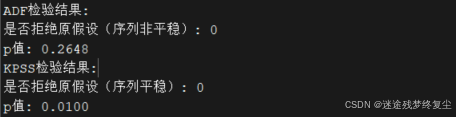
平稳性检验
- ADF检验:用于检测时间序列是否具有单位根,即是否非平稳。如果拒绝原假设(即h_adf=1),则认为序列平稳。
- KPSS检验:用于检测时间序列是否平稳。如果拒绝原假设(即h_kpss=0),则认为序列非平稳。
% 平稳性检验 - ADF检验
[h_adf, p_adf] = adftest(y);
fprintf('ADF检验结果:\n');
fprintf('是否拒绝原假设(序列非平稳): %d\n', h_adf);
fprintf('p值: %.4f\n', p_adf);
% 平稳性检验 - KPSS检验
[h_kpss, p_kpss] = kpsstest(y);
fprintf('KPSS检验结果:\n');
fprintf('是否拒绝原假设(序列平稳): %d\n', ~h_kpss);
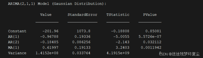
fprintf('p值: %.4f\n', p_kpss);强制确定模型
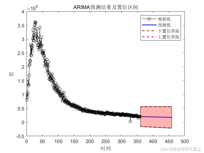
当强制确定模型,即isKill = 1时结果如下图所示:
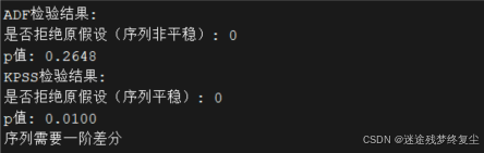
自动确定模型
当非强制确定模型时,会给出推荐的差分阶数,如下图所示:
差分(仅非强制确定模型时有效)
根据ADF和KPSS检验结果,确定差分阶数d。如果序列非平稳,则需要进行差分处理以使其平稳。
% 确定d参数
if isKill == 0
    % 根据ADF和KPSS检验结果确定d参数
    if h_adf == 1 && h_kpss == 0
        d = 0;
        disp('序列已经平稳')
    elseif h_adf == 0 && h_kpss == 1
        d = 1;
        disp('序列需要一阶差分')
    elseif h_adf == 1 && h_kpss == 1
        d = 2;
        disp('序列需要二阶差分')
    else
        error('无法确定d参数');
    end

    % 差分处理
    if d > 0
        y_diff = diff(train_data, d);
    else
        y_diff = train_data;
    end
else
    y_diff = train_data;
end
模型选择
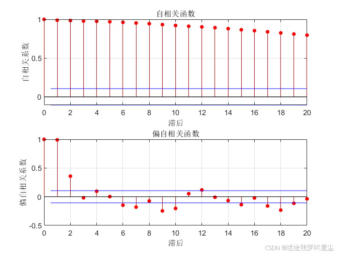
通过自相关函数(ACF)和偏自相关函数(PACF)图确定ARIMA模型的p和q参数。这里假设p=2和q=1。
% 确定p和q参数
figure
subplot(2,1,1)
autocorr(y_diff)
title('自相关函数')
xlabel('滞后')
ylabel('自相关系数')
subplot(2,1,2)
parcorr(y_diff)
title('偏自相关函数')
xlabel('滞后')
ylabel('偏自相关系数')
自动确定模型
运行结果如下图所示:

强制确定模型
运行结果如下图所示:
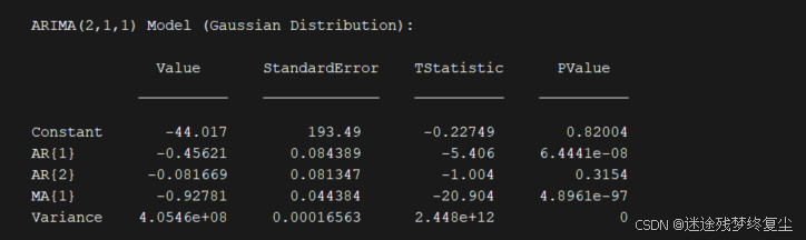
模型训练和预测
训练ARIMA模型并进行未来数据的预测,计算预测值的置信区间。
% 训练ARIMA模型
if isKill == 0
    model = arima('D', d, 'ARLags', [1 2], 'MALags', 1); % ARIMA(p, d, q) model
else
    model = arima(2, 1, 1);
end
model = estimate(model, y_diff);

% 测试未来时间预测情况
if isPre == 0
    horizon = length(y) - train_size;
else
    horizon = PreTime;
end
[forecastTest, YMSE, forecastCI] = forecast(model, horizon, 'Y0', y_diff);
ResultScale(:, 1) = forecastTest - 1.64*sqrt(YMSE); % 90%置信区间下限
ResultScale(:, 2) = forecastTest + 1.64*sqrt(YMSE); % 90%置信区间上限

% 自动确定的可能修正方法
if isKill == 0
    forecastTest = forecastTest + train_data(end) - forecastTest(1);
    ResultScale(:, 1) = forecastTest - 1.64*sqrt(YMSE); % 90%置信区间下限
    ResultScale(:, 2) = forecastTest + 1.64*sqrt(YMSE); % 90%置信区间上限
end

% 可视化预测结果
figure
plot(y, 'ko-')
hold on
if isPre == 0
    % 如果是测试数据预测,绘制测试集部分的预测值和置信区间
    time_axis = (train_size+1:length(y))';
    plot(time_axis, forecastTest, 'b-', 'LineWidth', 1.5)
    plot(time_axis, ResultScale(:, 1), 'r--', 'LineWidth', 1.5)
    plot(time_axis, ResultScale(:, 2), 'r--', 'LineWidth', 1.5)
    fill([time_axis; flipud(time_axis)], [ResultScale(:, 1); flipud(ResultScale(:, 2))], 'r', 'FaceAlpha', 0.3)
else
    % 如果是新时间段预测,绘制新时间段的预测值和置信区间
    time_axis = (length(y)+1:length(y)+PreTime)';
    plot(time_axis, forecastTest, 'b-', 'LineWidth', 1.5)
    plot(time_axis, ResultScale(:, 1), 'r--', 'LineWidth', 1.5)
    plot(time_axis, ResultScale(:, 2), 'r--', 'LineWidth', 1.5)
    fill([time_axis; flipud(time_axis)], [ResultScale(:, 1); flipud(ResultScale(:, 2))], 'r', 'FaceAlpha', 0.3)
end
xlabel('时间')
ylabel('值')
legend('观察值', '预测值', '下置信界限', '上置信界限')
title('ARIMA预测结果及置信区间')

% 误差分析和残差检验(仅当isPre == 0时)
if isPre == 0
    % 误差分析
    error = y(train_size+1:end) - forecastTest;
    mse = mean(error.^2);
    rmse = sqrt(mse);
    mae = mean(abs(error));

    fprintf('均方误差 (MSE): %.4f\n', mse);
    fprintf('均方根误差 (RMSE): %.4f\n', rmse);
    fprintf('平均绝对误差 (MAE): %.4f\n', mae);

    % 残差检验
    residuals = infer(model, y_diff);
    figure
    subplot(3,1,1)
    plot(residuals)
    xlabel('时间')
    ylabel('残差')
    title('残差')

    % 残差自相关检验
    subplot(3,1,2)
    autocorr(residuals)
    xlabel('滞后')
    ylabel('自相关系数')
    title('残差自相关函数')

    % 残差偏自相关检验
    subplot(3,1,3)
    parcorr(residuals)
    xlabel('滞后')
    ylabel('偏自相关系数')
    title('残差偏自相关函数')
end
自动确定模型
强制确定模型
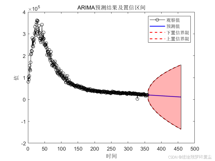
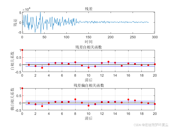
非预测模式
在非预测模式下,会给出相关参数的检验及可视化结果,如下图所示:

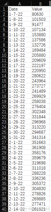
数据表格格式
【2024-08-05更新】数据表格格式如下:


 5098
5098

 被折叠的 条评论
为什么被折叠?
被折叠的 条评论
为什么被折叠?
 到【灌水乐园】发言


