import numpy as np
from sklearn.cluster import KMeans
from scipy.spatial.distance import cdist
import matplotlib.pyplot as plt
plt.rcParams['font.sans-serif']= ['SimHei']
plt.rcParams['axes.unicode_minus'] = False
cluster1 = np.random.uniform(0.5,1.5,(2,5))
cluster2 = np.random.uniform(3.5,4.5,(2,5))
X = np.hstack((cluster1,cluster2)).T
K = range(1, 6)
meandistortions = []
for k in K:
kmeans = KMeans(n_clusters=k)
kmeans.fit(X)
meandistortions.append(sum(np.min(cdist(X,kmeans.cluster_centers_,'euclidean'), axis=1)) / X.shape[0])
print("第 {} 次-聚类中心".format(k))
print(cdist(X,kmeans.cluster_centers_,'euclidean'))
print("第 {} 次聚类时----任一点到这{}个聚类中心其中一个的最小值".format(k,k))
print(np.min(cdist(X,kmeans.cluster_centers_,'euclidean'), axis=1))
print(meandistortions)
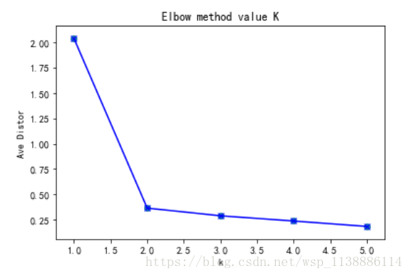
plt.plot(K, meandistortions,'bx-')
plt.xlabel('k')
plt.ylabel('Ave Distor')
plt.title('Elbow method value K')
plt.scatter(K,meandistortions)
第 1 次-聚类中心
[[1.74027894]
 [2.0994124 ]
 [2.19487598]
 [1.6247853 ]
 [2.5367581 ]
 [2.20055775]
 [2.38302686]
 [1.86944501]
 [1.76175722]
 [1.93239761]]
第 1 次聚类时----任一点到这1个聚类中心其中一个的最小值
[1.74027894 2.0994124  2.19487598 1.6247853  2.5367581  2.20055775
 2.38302686 1.86944501 1.76175722 1.93239761]
第 2 次-聚类中心
[[0.41437355 3.74440297]
 [0.48389576 4.08852385]
 [0.38539425 4.19780298]
 [0.39572757 3.6412047 ]
 [0.52902692 4.55253021]
 [4.20345795 0.38854537]
 [4.39984072 0.36626919]
 [3.88585126 0.15788191]
 [3.76106183 0.44396886]
 [3.9489673  0.0953715 ]]
第 2 次聚类时----任一点到这2个聚类中心其中一个的最小值
[0.41437355 0.48389576 0.38539425 0.39572757 0.52902692 0.38854537
 0.36626919 0.15788191 0.44396886 0.0953715 ]
第 3 次-聚类中心
[[0.81608013 3.74440297 0.14798486]
 [0.30865648 4.08852385 0.71166069]
 [0.66318639 4.19780298 0.36613121]
 [0.70939118 3.6412047  0.32438392]
 [0.30865648 4.55253021 0.76331617]
 [4.5077369  0.38854537 4.01019761]
 [4.6806729  0.36626919 4.22353482]
 [4.16439996 0.15788191 3.71276586]
 [4.01796009 0.44396886 3.6045836 ]
 [4.23428654 0.0953715  3.77060975]]
第 3 次聚类时----任一点到这3个聚类中心其中一个的最小值
[0.14798486 0.30865648 0.36613121 0.32438392 0.30865648 0.38854537
 0.36626919 0.15788191 0.44396886 0.0953715 ]
第 4 次-聚类中心
[[8.35275775e-01 3.74440297e+00 1.73347073e-01 6.54051405e-01]
 [1.11022302e-16 4.08852385e+00 7.07872006e-01 6.79497355e-01]
 [8.47523070e-01 4.19780298e+00 5.49196809e-01 2.96595119e-01]
 [6.03803237e-01 3.64120470e+00 1.73347073e-01 7.46038907e-01]
 [6.17312957e-01 4.55253021e+00 8.93632514e-01 2.96595119e-01]
 [4.29737222e+00 3.88545375e-01 3.84921905e+00 4.52767791e+00]
 [4.45158017e+00 3.66269187e-01 4.05533792e+00 4.73496134e+00]
 [3.93512012e+00 1.57881912e-01 3.54325021e+00 4.22253532e+00]
 [3.77486350e+00 4.43968859e-01 3.42992606e+00 4.10514152e+00]
 [4.00969435e+00 9.53714969e-02 3.60306131e+00 4.28280205e+00]]
第 4 次聚类时----任一点到这4个聚类中心其中一个的最小值
[1.73347073e-01 1.11022302e-16 2.96595119e-01 1.73347073e-01
 2.96595119e-01 3.88545375e-01 3.66269187e-01 1.57881912e-01
 4.43968859e-01 9.53714969e-02]
第 5 次-聚类中心
[[3.99547298e+00 6.54051405e-01 3.58249632e+00 8.35275775e-01
  1.73347073e-01]
 [4.37009505e+00 6.79497355e-01 3.90351785e+00 1.11022302e-16
  7.07872006e-01]
 [4.44684898e+00 2.96595119e-01 4.03676843e+00 8.47523070e-01
  5.49196809e-01]
 [3.90768915e+00 7.46038907e-01 3.46792299e+00 6.03803237e-01
  1.73347073e-01]
 [4.82002958e+00 2.96595119e-01 4.37759318e+00 6.17312957e-01
  8.93632514e-01]
 [2.10371686e-01 4.52767791e+00 5.75617138e-01 4.29737222e+00
  3.84921905e+00]
 [2.10371686e-01 4.73496134e+00 5.50736875e-01 4.45158017e+00
  4.05533792e+00]
 [4.68449304e-01 4.22253532e+00 6.68934761e-02 3.93512012e+00
  3.54325021e+00]
 [7.50566708e-01 4.10514152e+00 2.49346608e-01 3.77486350e+00
  3.42992606e+00]
 [3.69410477e-01 4.28280205e+00 1.82784602e-01 4.00969435e+00
  3.60306131e+00]]
第 5 次聚类时----任一点到这5个聚类中心其中一个的最小值
[1.73347073e-01 1.11022302e-16 2.96595119e-01 1.73347073e-01
 2.96595119e-01 2.10371686e-01 2.10371686e-01 6.68934761e-02
 2.49346608e-01 1.82784602e-01]
[2.034329515810916, 0.36604548812322546, 0.2907849769947618, 0.23919212137749707, 0.18596524433109082]
import numpy as np
from sklearn.cluster import KMeans
from sklearn import metrics
import matplotlib.pyplot as plt
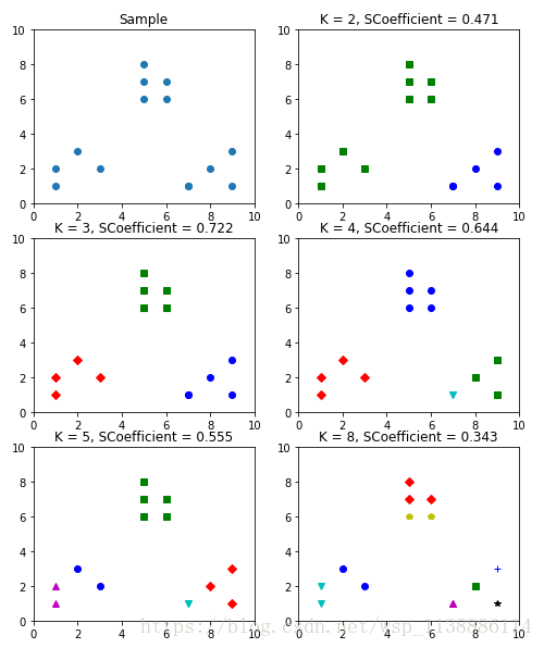
plt.figure(figsize=(8, 10))
plt.subplot(3, 2, 1)
x1 = np.array([1, 2, 3, 1, 5, 6, 5, 5, 6, 7, 8, 9, 7, 9])
x2 = np.array([1, 3, 2, 2, 8, 6, 7, 6, 7, 1, 2, 1, 1, 3])
X = np.array(list(zip(x1, x2))).reshape(len(x1), 2)
plt.xlim([0, 10])
plt.ylim([0, 10])
plt.title('Sample')
plt.scatter(x1, x2)
colors = ['b', 'g', 'r', 'c', 'm', 'y', 'k', 'b']
markers = ['o', 's', 'D', 'v', '^', 'p', '*', '+']
tests = [2, 3, 4, 5, 8]
subplot_counter = 1
for t in tests:
subplot_counter += 1
plt.subplot(3, 2, subplot_counter)
kmeans_model = KMeans(n_clusters=t).fit(X)
for i, l in enumerate(kmeans_model.labels_):
plt.plot(x1[i], x2[i], color=colors[l], marker=markers[l],ls='None')
plt.xlim([0, 10])
plt.ylim([0, 10])
plt.title('K = %s, SCoefficient = %.03f' % (t, metrics.silhouette_score
(X, kmeans_model.labels_,metric='euclidean')))
plt.show()
输出:
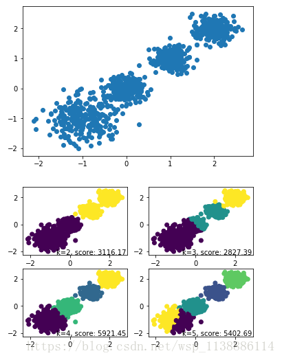
| 三、Mini Batch K-Means(适合大数据的聚类算法) |
import numpy as np
import matplotlib.pyplot as plt
from sklearn.cluster import MiniBatchKMeans, KMeans
from sklearn import metrics
from sklearn.datasets.samples_generator import make_blobs
X, y = make_blobs(n_samples=1000, n_features=2,
centers=[[-1,-1], [0,0], [1,1], [2,2]],
cluster_std=[0.4, 0.2, 0.2, 0.2],
random_state =9)
plt.scatter(X[:, 0], X[:, 1], marker='o')
plt.show()
for index, k in enumerate((2,3,4,5)):
plt.subplot(2,2,index+1)
y_pred = MiniBatchKMeans(n_clusters=k, batch_size = 200, random_state=9).fit_predict(X)
score= metrics.calinski_harabaz_score(X, y_pred)
plt.scatter(X[:, 0], X[:, 1], c=y_pred)
plt.text(.99, .01, ('k=%d, score: %.2f' % (k,score)),
transform=plt.gca().transAxes, size=10,
horizontalalignment='right')
plt.show()
输出:
print(__doc__)
import numpy as np
import matplotlib.pyplot as plt
from sklearn.cluster import KMeans
from sklearn.metrics import pairwise_distances_argmin
from sklearn.datasets import load_sample_image
from sklearn.utils import shuffle
from time import time
n_colors = 64
china = load_sample_image("china.jpg")
china = np.array(china, dtype=np.float64) / 255
w, h, d = original_shape = tuple(china.shape)
assert d == 3
image_array = np.reshape(china, (w * h, d))
print("一个小样本数据的拟合模型")
t0 = time()
image_array_sample = shuffle(image_array, random_state=0)[:1000]
kmeans = KMeans(n_clusters=n_colors, random_state=0).fit(image_array_sample)
print("done in %0.3fs." % (time() - t0))
print("Predicting color indices on the full image (k-means)")
t0 = time()
labels = kmeans.predict(image_array)
print("done in %0.3fs." % (time() - t0))
def recreate_image(codebook, labels, w, h):
d = codebook.shape[1]
image = np.zeros((w, h, d))
label_idx = 0
for i in range(w):
for j in range(h):
image[i][j] = codebook[labels[label_idx]]
label_idx += 1
return image
plt.figure(1)
plt.clf()
ax = plt.axes([0, 0, 1, 1])
plt.axis('off')
plt.title('Original image (96,615 colors)')
plt.imshow(china)
plt.figure(2)
plt.clf()
ax = plt.axes([0, 0, 1, 1])
plt.axis('off')
plt.title('Quantized image (64 colors, K-Means)')
plt.imshow(recreate_image(kmeans.cluster_centers_, labels, w, h))
plt.show()
输出:
-
一个小样本数据的拟合模型
done in 0.463s.
Predicting color indices on the full image (k-means)
done in 0.189s.


 281
281

 被折叠的 条评论
为什么被折叠?
被折叠的 条评论
为什么被折叠?
 到【灌水乐园】发言


