深度学习之卷积神经网络(代码可直接运行)

深度学习之卷积神经网络

图像卷积运算

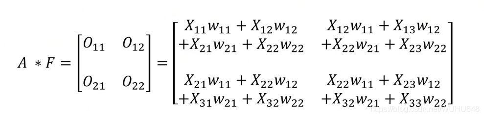
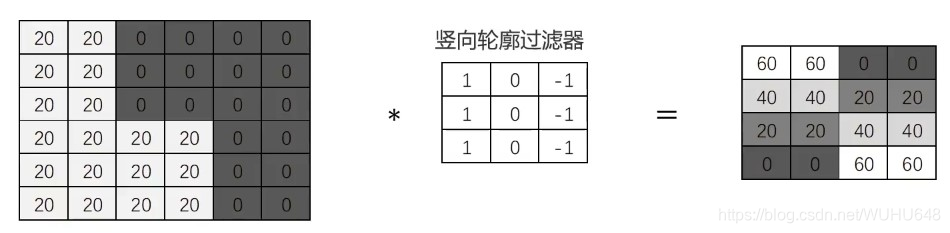
对图像矩阵与滤波器矩阵进行对应相乘再求和运算，转化得到新的矩阵。作用:快速定位图像中某些边缘特征
英文: convolution
CNN
A与B的卷积通常表示为:A*B或convolution(A,B)
···· X11 X12 X13
A= X21 X22 X23
···· X31 X32 X33
····
F= W11 W12
···· W21 W22


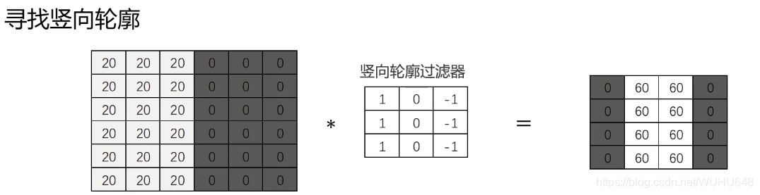
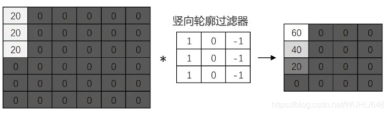
包含竖向轮廓的区域非常亮(灰度值高)

计算机根据样本图片，自动寻找合适的轮廓过滤器，对新图片进行轮廓匹配
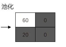
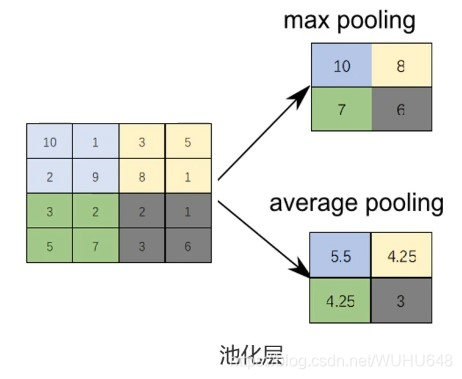
池化:按照一个固定规则对图像矩阵进行处理，将其转换为更低维度的矩阵
最大法池化(Max-pooling)

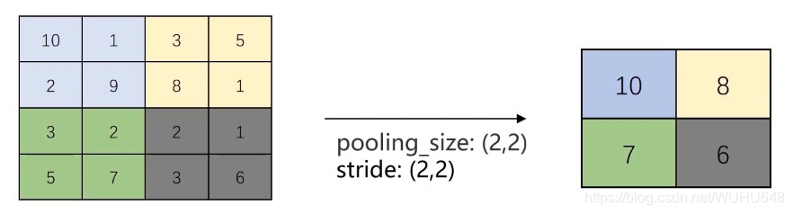
Stride为窗口滑动步长，用于池化、卷积的计算中。
保留核心信息的情况下，实现维度缩减
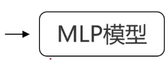
把卷积、池化、mlp先后连接在一起，组成卷积神经网络。


作用:
1、使部分神经元为0，防止过拟合
2、助于模型的求解
Relu函数:f(x) = max(x, 0)

转化成全连接层

卷积神经网络两大特点：

参数共享(parameter sharing):同一个特征过滤器可用于整张图片
稀疏连接(sparsity of connections):生成的特征图片每个节点只与原图片中特定节点连接



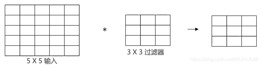
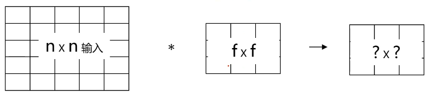
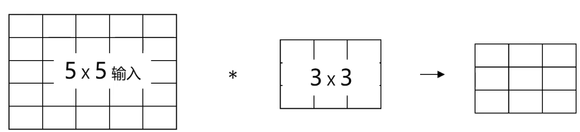
？×？=（n-f+1）×(n-f+1)
卷积运算导致的两个问题:
图像被压缩，造成信息丢失
边缘信息使用少，容易被忽略
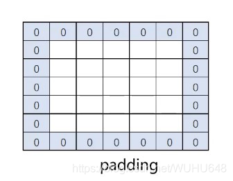
图像填充(padding)
通过在图像各边增加像素，使其在进行卷积运算后维持原图大小


通过padding增加像素的数量，由过滤器尺寸与stride决定
在这里插入图片描述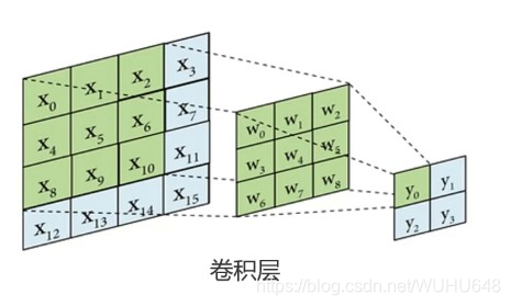

经典的CNN模型

1、参考经典的CNN结构搭建新模型
2、使用经典的CNN模型结构对图像预处理，再建立MLP模型
经典的CNN模型:
LeNet-5

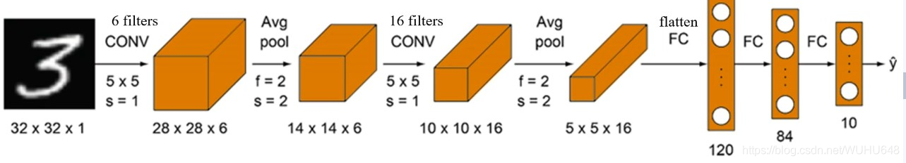
（1）6个5×5的过滤器滑动窗口为1
（2）平均值池化：2×2的滑动窗口是2
（3）16个5×5的过滤器滑动窗口为1
（4）池化：2×2的滑动窗口是2
（5）展开
（6）进行MLP模型
（7）输出10个类别
输入图像:32 X 32灰度图，1个通道(channel)训练参数:约60,000个
特点:
1、随着网络越深，图像的高度和宽度在缩小，通道数在增加
2、卷积与池化先后成对使用
AlexNet

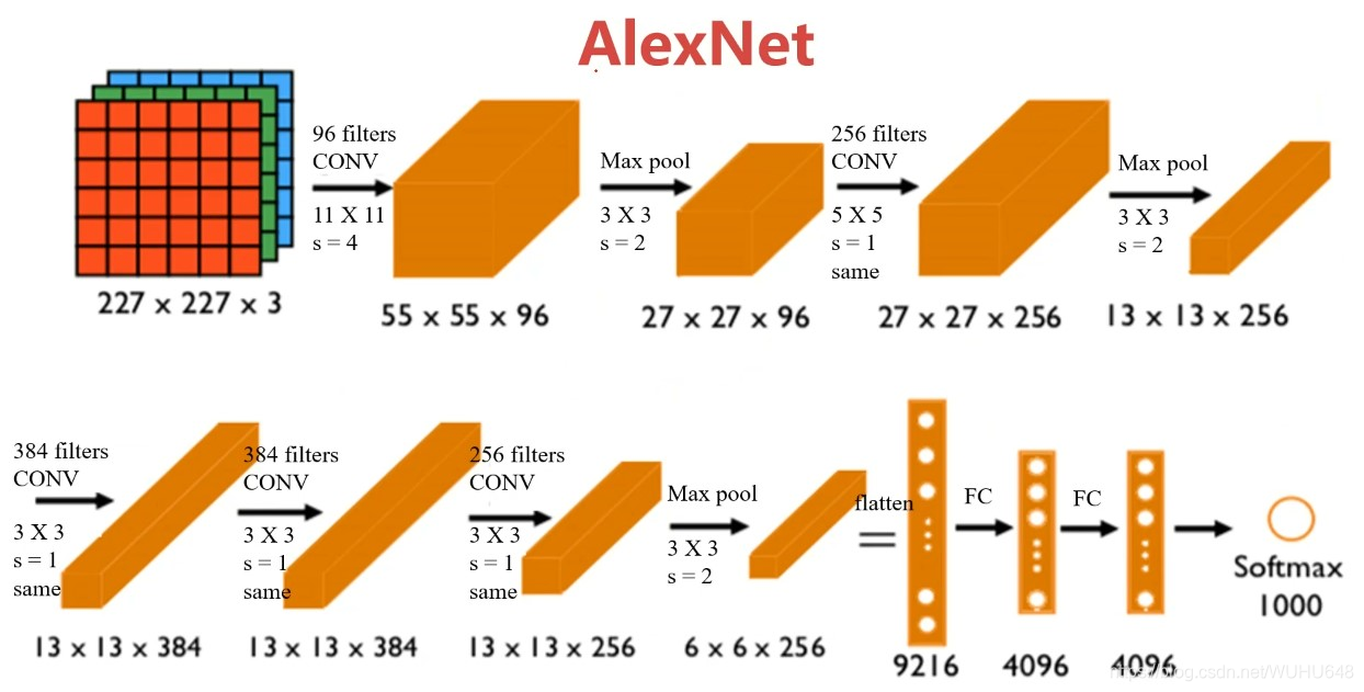
（1）96个11×11的过滤器滑动窗口为4
（2）最大值池化：3×3的滑动窗口是2
（3）256个5×5的过滤器滑动窗口为1
（4）最大值池化：3×3的滑动窗口是2
…
（n）输出1000个类别
输入图像:227X 227X 3 RGB图，3个通道训练参数:约60,000,000个
特点:
1、适用于识别较为复杂的彩色图，可识别1000种类别
2、结构比LeNet更为复杂，使用Relu作为激活函数
学术界开始相信深度学习技术,
在计算机视觉应用中可以得到很不错的结果。
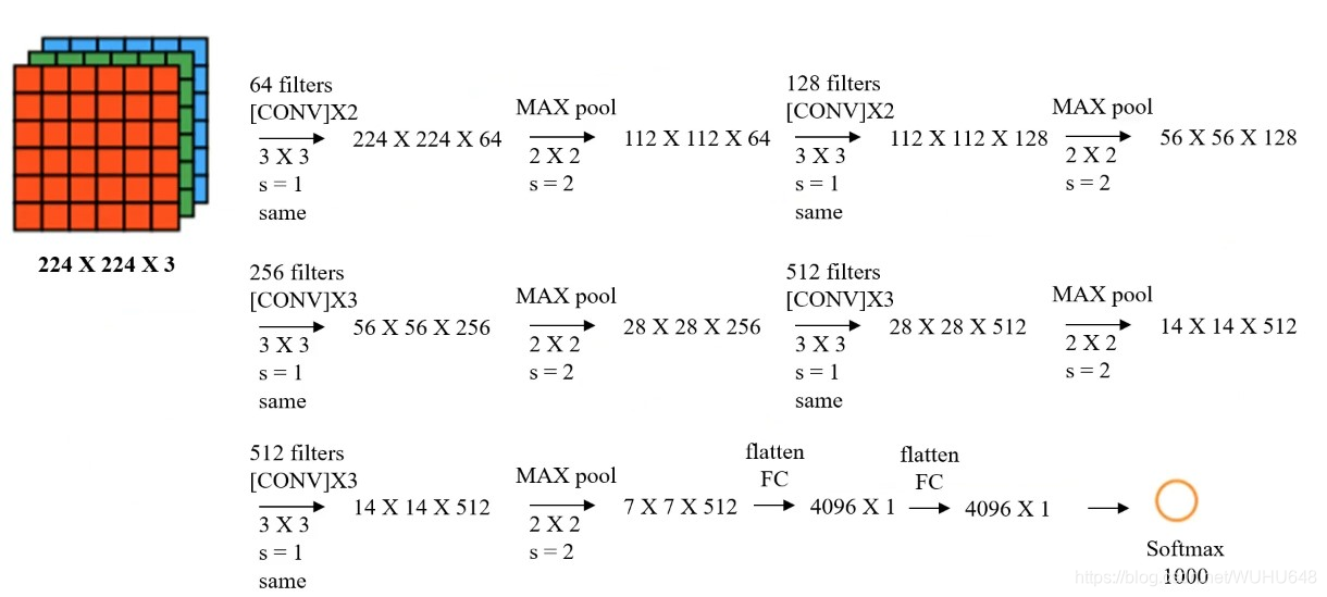
VGG




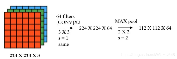
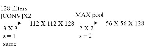
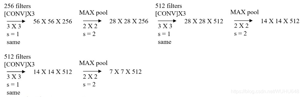
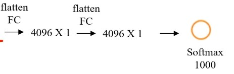
所有的卷积都是64个3×3的过滤器移动窗口是1，最大值池化：2×2的滑动窗口是2
不断重复同样的步骤
输入图像: 227 X 227X 3 RGB图，3个通道训练参数:约138,000,000个
特点:
1、所有卷积层filter 宽和高都是3，步长为1,padding 都使用same convolution;
2、所有池化层的 filter 宽和高都是2，步长都是2;
3、相比alexnet，有更多的filter用于提取轮廓信息，具有更高精准性
经典的CNN模型用于新场景
1、使用经典的CNN模型结构对图像预处理，再建立MLP模型;
（1）加载经典的CNN模型，剥除其FC层，对图像进行预处理
（2）把预处理完成的数据作为输入，分类结果为输出，建立一个mlp模型
（3）模型训练
2、参考经典的CNN结构搭建新模型

实战代码如下：

实战一：
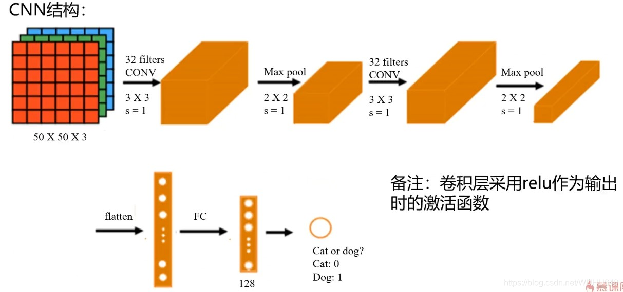
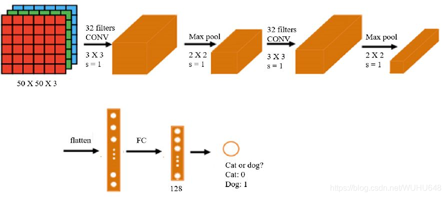
基于dataset\training_set数据，根据提供的结构，建立CNN模型，识别图片中的猫/狗，计算预测准确率：
1.识别图片中的猫/狗、计算dataset\test_set测试数据预测准确率
2.从网站下载猫/狗图片，对其进行预测

#load the data
from keras.preprocessing.image import ImageDataGenerator#图片加载
train_datagen = ImageDataGenerator(rescale=1./255)#图片预处理
#加载出图片
training_set = train_datagen.flow_from_directory('./dataset/training_set',target_size=(50,50),batch_size=32,class_mode='binary')
#路径   像素大小（50,50）   每次选择32张图片   模式选择二分类binary
#set up the cnn model
from keras.models import Sequential
from keras.layers import Conv2D, MaxPool2D, Flatten, Dense#卷积层  池化层  图像的展开    

model = Sequential()
#卷积层
model.add(Conv2D(32,(3,3),input_shape=(50,50,3),activation='relu'))#32个3×3
#池化层
model.add(MaxPool2D(pool_size=(2,2)))#2×2  移动窗口是1
#卷积层
model.add(Conv2D(32,(3,3),activation='relu'))
#池化层
model.add(MaxPool2D(pool_size=(2,2)))
#flattening layer
model.add(Flatten())#转化成展开
#FC layer
model.add(Dense(units=128,activation='relu'))#隐藏层
model.add(Dense(units=1,activation='sigmoid'))#输出层
#configure the model
model.compile(optimizer='adam',loss='binary_crossentropy',metrics=['accuracy'])
model.summary()#模型结构

Model: “sequential_2”

---

Layer (type) Output Shape Param #

conv2d_3 (Conv2D) (None, 48, 48, 32) 896

---

max_pooling2d_3 (MaxPooling2 (None, 24, 24, 32) 0

---

conv2d_4 (Conv2D) (None, 22, 22, 32) 9248

---

max_pooling2d_4 (MaxPooling2 (None, 11, 11, 32) 0

---

flatten_2 (Flatten) (None, 3872) 0

---

dense_3 (Dense) (None, 128) 495744

---

dense_4 (Dense) (None, 1) 129

Total params: 506,017 Trainable params: 506,017 Non-trainable params: 0

---

#train the model
model.fit_generator(training_set,epochs=20)#迭代20次
#accuracy on the training data
accuracy_train = model.evaluate_generator(training_set)#计算准确率
print(accuracy_train)
#accuracy on the test data
test_set = train_datagen.flow_from_directory('./dataset/test_set',target_size=(50,50),batch_size=32,class_mode='binary')
accuracy_test = model.evaluate_generator(test_set)
print(accuracy_test)

训练准确率为100%测试准确率为76%，对于二分类50%的准确率来说，此模型的还是可以来进行使用的

#load single image
from keras.preprocessing.image import load_img, img_to_array
pic_dog = 'dog.jpg'
pic_dog = load_img(pic_dog,target_size=(50,50))
pic_dog = img_to_array(pic_dog)
pic_dog = pic_dog/255
pic_dog = pic_dog.reshape(1,50,50,3)
result = model.predict_classes(pic_dog)
print(result)

[[1]]代码预测的是小狗

pic_cat = 'cat1.jpg'
pic_cat = load_img(pic_cat,target_size=(50,50))
pic_cat = img_to_array(pic_cat)
pic_cat = pic_cat/255
pic_cat = pic_cat.reshape(1,50,50,3)
result = model.predict_classes(pic_cat)
print(result)

[[0]]代码预测的是小猫

training_set.class_indices

{‘cats’: 0, ‘dogs’: 1}

# make prediction on multiple images
import matplotlib as mlp
font2 = {'family' : 'SimHei',
'weight' : 'normal',
'size'   : 20,
}
mlp.rcParams['font.family'] = 'SimHei'
mlp.rcParams['axes.unicode_minus'] = False
from matplotlib import pyplot as plt
from matplotlib.image import imread
from keras.preprocessing.image import load_img
from keras.preprocessing.image import img_to_array
from keras.models import load_model
a = [i for i in range(1,10)]
fig = plt.figure(figsize=(10,10))
for i in a:
    img_name = str(i)+'.jpg'
    img_ori = load_img(img_name, target_size=(50, 50))
    img = img_to_array(img_ori)
    img = img.astype('float32')/255
    img = img.reshape(1,50,50,3)
    result = model.predict_classes(img)
    img_ori = load_img(img_name, target_size=(250, 250))
    plt.subplot(3,3,i)
    plt.imshow(img_ori)
    plt.title('预测为：狗狗' if result[0][0] == 1 else '预测为：猫咪')
plt.show()

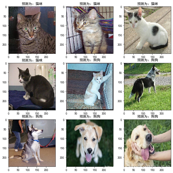
从上述结果来看，只有最中间的一幅小猫的图片被预测成小狗的错误，其他预测都是准确的。
实战二：
使用VGG16的结构提取图像特征，再根据特征建立mlp模型，实现猫狗图像识别。训练/测试数据：dataset\data_vgg：
1.对数据进行分离、计算测试数据预测准确率
2.从网站下载猫/狗图片，对其进行预测
mlp模型一个隐藏层，10个神经元

#load the data
from keras.preprocessing.image import load_img,img_to_array
img_path = '1.jpg'
img = load_img(img_path,target_size=(224,224))#希望加载进来的像素大小是224*224
img = img_to_array(img)
type(img)

from keras.applications.vgg16 import VGG16
from keras.applications.vgg16 import preprocess_input
import numpy as np
model_vgg = VGG16(weights='imagenet',include_top=False)#去掉全连接层
x = np.expand_dims(img,axis=0)
x = preprocess_input(x)#可以把图片矩阵转化成可用于VGG16输入的矩阵
#特征提取
features = model_vgg.predict(x)
#flatten
features = features.reshape(1,7*7*512)
#visualize the data
%matplotlib inline
from matplotlib import pyplot as plt
fig = plt.figure(figsize=(5,5))
img = load_img(img_path,target_size=(224,224))
plt.imshow(img)

#load image and preprocess it with vgg16 structure
#--by flare
from keras.preprocessing.image import img_to_array,load_img
from keras.applications.vgg16 import VGG16
from keras.applications.vgg16 import preprocess_input
import numpy as np

model_vgg = VGG16(weights='imagenet', include_top=False)
#define a method to load and preprocess the image
def modelProcess(img_path,model):
    img = load_img(img_path, target_size=(224, 224))
    img = img_to_array(img)
    x = np.expand_dims(img,axis=0)
    x = preprocess_input(x)
    x_vgg = model.predict(x)
    x_vgg = x_vgg.reshape(1,25088)
    return x_vgg
#list file names of the training datasets
import os
folder = "dataset/data_vgg/cats"
dirs = os.listdir(folder)
#generate path for the images
img_path = []
for i in dirs:                             
    if os.path.splitext(i)[1] == ".jpg":   
        img_path.append(i)
img_path = [folder+"//"+i for i in img_path]

#preprocess multiple images
features1 = np.zeros([len(img_path),25088])
for i in range(len(img_path)):
    feature_i = modelProcess(img_path[i],model_vgg)
    print('preprocessed:',img_path[i])
    features1[i] = feature_i
    
folder = "dataset/data_vgg/dogs"
dirs = os.listdir(folder)
img_path = []
for i in dirs:                             
    if os.path.splitext(i)[1] == ".jpg":   
        img_path.append(i)
img_path = [folder+"//"+i for i in img_path]
features2 = np.zeros([len(img_path),25088])
for i in range(len(img_path)):
    feature_i = modelProcess(img_path[i],model_vgg)
    print('preprocessed:',img_path[i])
    features2[i] = feature_i
    
#label the results
print(features1.shape,features2.shape)
y1 = np.zeros(300)
y2 = np.ones(300)

#generate the training data
X = np.concatenate((features1,features2),axis=0)
y = np.concatenate((y1,y2),axis=0)
y = y.reshape(-1,1)
#split the training and test data
from sklearn.model_selection import train_test_split
X_train,X_test,y_train,y_test = train_test_split(X,y,test_size=0.3,random_state=50)
#set up the mlp model
from keras.models import Sequential
from keras.layers import Dense
model = Sequential()
model.add(Dense(units=10,activation='relu',input_dim=25088))
model.add(Dense(units=1,activation='sigmoid'))
model.summary()

Model: “sequential_1” _________________________________________________________________ Layer (type) Output Shape Param # ================================================================= dense_1 (Dense) (None, 10) 250890 _________________________________________________________________ dense_2 (Dense) (None, 1) 11 ================================================================= Total params: 250,901 Trainable params: 250,901 Non-trainable params: 0 _________________________________________________________________

#configure the model
model.compile(optimizer='adam',loss='binary_crossentropy',metrics=['accuracy'])
#train the model
model.fit(X_train,y_train,epochs=50)
from sklearn.metrics import accuracy_score
y_train_predict = model.predict_classes(X_train)
accuracy_train = accuracy_score(y_train,y_train_predict)
print(accuracy_train)
#测试准确率
y_test_predict = model.predict_classes(X_test)
accuracy_test = accuracy_score(y_test,y_test_predict)
print(accuracy_test)

训练准确率为98.57%测试准确率为97.78%，两者准确率都是非常高的，而且要比实战一中的模型预测要更加准。

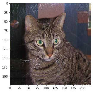
img_path = 'myself_cat.jpg'
img = load_img(img_path,target_size=(224,224))
img = img_to_array(img)
x = np.expand_dims(img,axis=0)
x = preprocess_input(x)
features = model_vgg.predict(x)
features = features.reshape(1,7*7*512)
result = model.predict_classes(features)
print(result)

[[0]]
可以看出预测的结果是正确的

# coding:utf-8
import matplotlib as mlp
font2 = {'family' : 'SimHei',
'weight' : 'normal',
'size'   : 20,
}
mlp.rcParams['font.family'] = 'SimHei'
mlp.rcParams['axes.unicode_minus'] = False
from matplotlib import pyplot as plt
from matplotlib.image import imread
from keras.preprocessing.image import load_img
from keras.preprocessing.image import img_to_array
from keras.models import load_model
#from cv2 import load_img
a = [i for i in range(1,10)]
fig = plt.figure(figsize=(10,10))
for i in a:
    img_name = str(i)+'.jpg'
    img_path = img_name
    img = load_img(img_path, target_size=(224, 224))
    img = img_to_array(img)
    x = np.expand_dims(img,axis=0)
    x = preprocess_input(x)
    x_vgg = model_vgg.predict(x)
    x_vgg = x_vgg.reshape(1,25088)
    result = model.predict_classes(x_vgg)
    img_ori = load_img(img_name, target_size=(250, 250))
    plt.subplot(3,3,i)
    plt.imshow(img_ori)
    plt.title('预测为：狗狗' if result[0][0] == 1 else '预测为：猫咪')
plt.show()