经验模式分解理论及其应用

经验模式分解基础理论

$\hspace{0.5cm}$ 经验模式分解（Empirical mode decomposition ,EMD) is a nonlinear signal processing method developed by Huang et al. It can decompose a signal into a sum of functions, intrinsic mode functions (IMFs)。这些 IMFs必须满足两个条件： (1) the number of extrema and the number of zero-crossings either are equal or differ at the most by one; (2) the mean value of the envelope defined by the local maxima and the local minima is zero at all points.
$\hspace{0.5cm}$ 时间序列 x(t)的详细分解过程可概括为如下：
$\hspace{0.5cm}$(1) Identify all the local maxima and local minima of x(t), obtain the lower envelope $x_l(t)$ and the upper envelope $x_u(t)$ by interpolate the local minima and the local maxima, calculate the mean $m1=(x_l(t)+x_u(t))/2$.
$\hspace{0.5cm}$(2) Extract the details, $h_1 = x(t)-m1$, check the properties of $h_1$, if $h_1$ satisfies conditions $r$ and $s$ above, then $c_1 = h_1$, an IMF is derived; if $h_1$ is not an IMF, replace $x(t)$ with $h_1$, repeat step (1)$~$(2) until it satisfies the stop conditions $r$ and $s$ above.
$\hspace{0.5cm}$ (3) Regard $r = x(t) - h_1$ as a new $x(t)$, the steps are applied repeatedly to $\hspace{0.5cm}$ the residue in order to obtain the second, the third and nth IMF until a predetermined threshold is achieved, or until the residue becomes a monotonic function.
$\hspace{0.5cm}$ 时间序列好的数据 $x(t)$ 可以表示为 IMFs 与余差之和：

$$x(t)=\sum_{i=1}^{n}c_i+r$$
$\hspace{0.5cm}$其中， $n$是IMFs的个数；$c_i(i = 1,2,\cdots,n)$为IMFs,它们互相之前是近似正交的； $r$ 是最终的余差，代表着$x(t)$的主要趋势。

使用MATLAB进行EMD分解

---

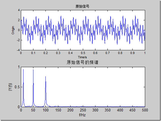
原始信号由3个正弦信号加噪声组成，如下

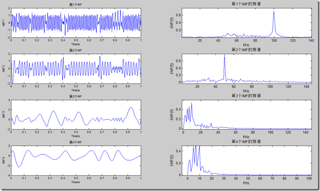
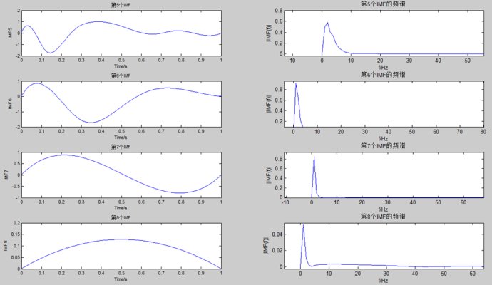
下面为做EMD分解的结果


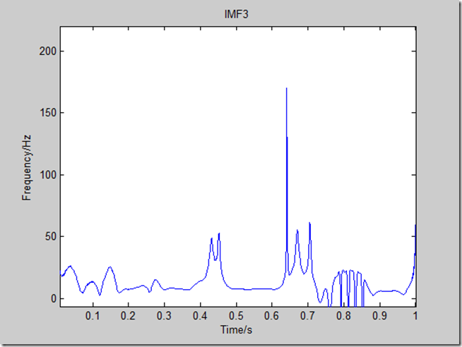
第三次分解信号的瞬时频率如下

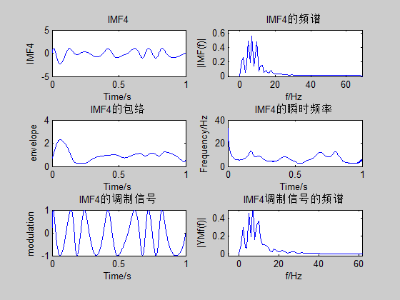
第四次分解信号的Hilbert分析

具体代码如下
test.m文件

clc
clear all
close all
% [x, Fs] = wavread('Hum.wav');
% Ts = 1/Fs;
% x = x(1:6000);
Ts = 0.001;
Fs = 1/Ts;
t=0:Ts:1;
x = sin(2*pi*10*t) + sin(2*pi*50*t) + sin(2*pi*100*t) + 0.1*randn(1, length(t));
imf = emd(x);
plot_hht(x,imf,1/Fs);
k = 4;
y = imf{k};
N = length(y);
t = 0:Ts:Ts*(N-1);
[yenvelope, yfreq, yh, yangle] = HilbertAnalysis(y, 1/Fs);
yModulate = y./yenvelope;
[YMf, f] = FFTAnalysis(yModulate, Ts);
Yf = FFTAnalysis(y, Ts);
figure
subplot(321)
plot(t, y)
title(sprintf('IMF%d', k))
xlabel('Time/s')
ylabel(sprintf('IMF%d', k));
subplot(322)
plot(f, Yf)
title(sprintf('IMF%d的频谱', k))
xlabel('f/Hz')
ylabel('|IMF(f)|');
subplot(323)
plot(t, yenvelope)
title(sprintf('IMF%d的包络', k))
xlabel('Time/s')
ylabel('envelope');
subplot(324)
plot(t(1:end-1), yfreq)
title(sprintf('IMF%d的瞬时频率', k))
xlabel('Time/s')
ylabel('Frequency/Hz');
subplot(325)
plot(t, yModulate)
title(sprintf('IMF%d的调制信号', k))
xlabel('Time/s')
ylabel('modulation');
subplot(326)
plot(f, YMf)
title(sprintf('IMF%d调制信号的频谱', k))
xlabel('f/Hz')
ylabel('|YMf(f)|');

findpeaks.m文件
function n = findpeaks(x)
% Find peaks. 找极大值点，返回对应极大值点的坐标
n    = find(diff(diff(x) > 0) < 0); % 相当于找二阶导小于0的点
u    = find(x(n+1) > x(n));
n(u) = n(u)+1;                      % 加1才真正对应极大值点
% 图形解释上述过程
% figure
% subplot(611)
% x = x(1:100);
% plot(x, '-o')
% grid on
%
% subplot(612)
% plot(1.5:length(x), diff(x) > 0, '-o')
% grid on
% axis([1,length(x),-0.5,1.5])
%
% subplot(613)
% plot(2:length(x)-1, diff(diff(x) > 0), '-o')
% grid on
% axis([1,length(x),-1.5,1.5])
%
% subplot(614)
% plot(2:length(x)-1, diff(diff(x) > 0)<0, '-o')
% grid on
% axis([1,length(x),-1.5,1.5])
%
% n    = find(diff(diff(x) > 0) < 0);
% subplot(615)
% plot(n, ones(size(n)), 'o')
% grid on
% axis([1,length(x),0,2])
%
% u    = find(x(n+1) > x(n));
% n(u) = n(u)+1;
% subplot(616)
% plot(n, ones(size(n)), 'o')
% grid on
% axis([1,length(x),0,2])

plot_hht.m文件

function plot_hht(x,imf,Ts)
% Plot the HHT.
% :: Syntax`这里写代码片`
%    The array x is the input signal and Ts is the sampling period.
%    Example on use: [x,Fs] = wavread('Hum.wav');
%                    plot_hht(x(1:6000),1/Fs);
% Func : emd
% imf = emd(x);
for k = 1:length(imf)
    b(k) = sum(imf{k}.*imf{k});
    th   = unwrap(angle(hilbert(imf{k})));  % 相位
    d{k} = diff(th)/Ts/(2*pi);          % 瞬时频率
end
[u,v] = sort(-b);
b     = 1-b/max(b);                     % 后面绘图的亮度控制
% Hilbert瞬时频率图
N = length(x);
c = linspace(0,(N-2)*Ts,N-1);           % 0:Ts:Ts*(N-2)
for k = v(1:2)                          % 显示能量最大的两个IMF的瞬时频率
    figure
    plot(c,d{k});
    xlim([0 c(end)]);
    ylim([0 1/2/Ts]);
    xlabel('Time/s')
    ylabel('Frequency/Hz');
    title(sprintf('IMF%d', k))
end
% 显示各IMF
M = length(imf);
N = length(x);
c = linspace(0,(N-1)*Ts,N);             % 0:Ts:Ts*(N-1)
for k1 = 0:4:M-1
    figure
    for k2 = 1:min(4,M-k1)
        subplot(4,2,2*k2-1)
        plot(c,imf{k1+k2})
        set(gca,'FontSize',8,'XLim',[0 c(end)]);
        title(sprintf('第%d个IMF', k1+k2))
        xlabel('Time/s')
        ylabel(sprintf('IMF%d', k1+k2));

        subplot(4,2,2*k2)
        [yf, f] = FFTAnalysis(imf{k1+k2}, Ts);
        plot(f, yf)
        title(sprintf('第%d个IMF的频谱', k1+k2))
        xlabel('f/Hz')
        ylabel('|IMF(f)|');
    end
end
figure
subplot(211)
plot(c,x)
set(gca,'FontSize',8,'XLim',[0 c(end)]);
title('原始信号')
xlabel('Time/s')
ylabel('Origin');
subplot(212)
[Yf, f] = FFTAnalysis(x, Ts);
plot(f, Yf)
title('原始信号的频谱')
xlabel('f/Hz')
ylabel('|Y(f)|');
emd.m文件
function imf = emd(x)
% Empiricial Mode Decomposition (Hilbert-Huang Transform)
% EMD分解或HHT变换
% 返回值为cell类型，依次为一次IMF、二次IMF、...、最后残差
x   = transpose(x(:));
imf = [];
while ~ismonotonic(x)
    x1 = x;
    sd = Inf;
    while (sd > 0.1) || ~isimf(x1)
        s1 = getspline(x1);         % 极大值点样条曲线
        s2 = -getspline(-x1);       % 极小值点样条曲线
        x2 = x1-(s1+s2)/2;

        sd = sum((x1-x2).^2)/sum(x1.^2);
        x1 = x2;
    end

    imf{end+1} = x1;
    x          = x-x1;
end
imf{end+1} = x;
% 是否单调
function u = ismonotonic(x)
u1 = length(findpeaks(x))*length(findpeaks(-x));
if u1 > 0
    u = 0;
else
    u = 1;
end
% 是否IMF分量
function u = isimf(x)
N  = length(x);
u1 = sum(x(1:N-1).*x(2:N) < 0);                     % 过零点的个数
u2 = length(findpeaks(x))+length(findpeaks(-x));    % 极值点的个数
if abs(u1-u2) > 1
    u = 0;
else
    u = 1;
end
% 据极大值点构造样条曲线
function s = getspline(x)
N = length(x);
p = findpeaks(x);
s = spline([0 p N+1],[0 x(p) 0],1:N);
FFTAnalysis.m文件
% 频谱分析
function [Y, f] = FFTAnalysis(y, Ts)
Fs = 1/Ts;
L = length(y);
NFFT = 2^nextpow2(L);
y = y - mean(y);
Y = fft(y, NFFT)/L;
Y = 2*abs(Y(1:NFFT/2+1));
f = Fs/2*linspace(0, 1, NFFT/2+1);
end
HilbertAnalysis.m文件
% Hilbert分析
function [yenvelope, yf, yh, yangle] = HilbertAnalysis(y, Ts)
yh = hilbert(y);
yenvelope = abs(yh);                % 包络
yangle = unwrap(angle(yh));         % 相位
yf = diff(yangle)/2/pi/Ts;          % 瞬时频率
end